Download
1 / 47
480 likes | 653 Views
Tools for Preprocessing Mass Spectrometry Data. Utah State University – Spring 2012 STAT 5570: Statistical Bioinformatics Notes 5.1. 1. Outline. Introduction to Mass Spectrometry Issues in Preprocessing Recent Software Tools Sample Analysis Misc. Notes. 2. Mass Spectrometry.

E N D
Tools for Preprocessing Mass Spectrometry Data Utah State University – Spring 2012 STAT 5570: Statistical Bioinformatics Notes 5.1 1
Outline • Introduction to Mass Spectrometry • Issues in Preprocessing • Recent Software Tools • Sample Analysis • Misc. Notes 2
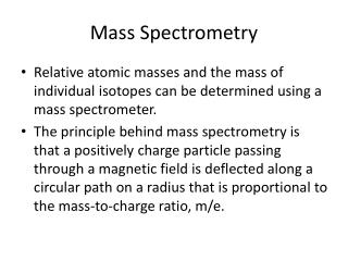
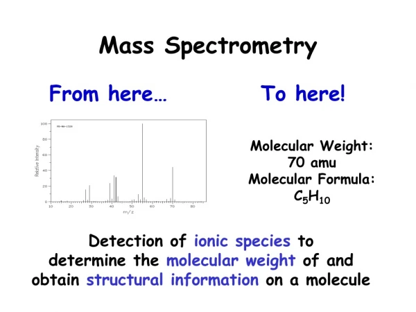
Mass Spectrometry • Technology to assess composition of a complex mixture of proteins and metabolites • MALDI: matrix-assisted laser desorption and ionization • Biological sample mixed with a crystal-forming energy-absorbing matrix (EAM) • Mixture crystallizes on metal plate (chip or slide) • In a vacuum, plate hit with pulses from laser • Molecules in matrix are released, producing a gas plume of ions • Electric field accelerates ions into a flight tube towards a detector, recording time of flight 3 (Dijkstra 2008; Coombes et al. 2007)
SELDI-TOF • Surface-enhanced laser desorption and ionization • Special case of MALDI • Ciphergen (Bio-Rad) ProteinChip: eight-spot array • Surface of metal plate chemically modified to favor particular classes of proteins (Coombes et al. 2007; Tibshirani et al. 2004; image from www.pasteur.fr)
SELDI ProteinChip Technology • Within narrow time intervals (1-4 nanoseconds), detector records the number of particles: time of flight • Animation www.learner.org/channel/courses/biology/archive/animations/hires/a_proteo3_h.html (Coombes et al. 2007; Tibshirani et al. 2004; image from Yasui et al. 2003)
Other Separation Techniques • Gas Chromatography (GC) • also called gas-liquid chromatography • Liquid Chromatography (LC) • also called high performance liquid chromatography (HPLC) • Common Features: • molecules pass through a chromatographic column • time of passage depends on molecule characteristics • coupled with a detector to record time-of-flight and report mass spectra (GC-MS, LC-MS) • Successful separation reduces number of overlapping peaks (Dijkstra 2008)
Mass-to-charge (m/z) ratio • Each molecule has a mass (m) and a charge (z) • The m/z ratio affects the molecule’s velocity in the flight tube, and consequently its time of flight t • Based on the law of energy conservation: • Parameters t0, α, and β estimated using [instrument-specific] calibration data; V is electronvolt unit of energy (Dijkstra 2008)
Two-Step Analysis Approach • 1. Preprocess Mass Spectrometry Data • Identify peak locations and quantify each peak in each spectrum • (1.5). Identify Components • Determine which molecule (protein, metabolite) caused each peak • 2. Test for Differences • Similar to differential expression of genes between treatment and control (Morris et al. 2005; Coombes et al. 2007)
Preprocessing Issues • Calibration • Filtering / Denoise Spectra • Detrend / Remove Baseline from Spectra • Normalization of Multiple Spectra • Peak Detection • Peak Alignment • Peak Quantification (Coombes et al. 2007)
Calibration • Mapping observed time-of-flight to m/z values • Experimentally: • create a sample containing a small number of [mass known] proteins • obtain spectrum from sample using the mass spectrometry instrument • Parameters t0, α, and β estimated using [instrument-specific] calibration data: • Also refers to finding common m/z values for multiple spectra (msPrepare function uses linear interpolation) (Dijkstra 2008; Coombes et al. 2007; Morris et al. 2005)
Preprocessing Strategies • Choices: • How to approach each preprocessing issue • Order of addressing each preprocessing issue • Some available software • Commercial – usually manufacturer-specific • R Packages • msProcess (CRAN: Lixin Gong) – examples used here • PROcess (Bioconductor: Xiaochun Li) • caMassClass (CRAN: JarekTuszynski) • MassSpecWavelet (Bioconductor: Pan Du) • FTICRMS (CRAN: Don Barkauskas) • RProteomics (caBIG: Rich Haney)
Sample Data and Code • Reproducibility of results in these slides • R code included in these slides • R Package msBreast: dataset of 96 protein mass spectra generated from a pooled sample of nipple aspirate fluid (NAF) from healthy breasts and breasts with cancer • Observations with m/z below 950 eliminated • just noise from matrix molecules • these observations can be just saturation (too many ions hitting the detector so it can’t count them) (Coombes et al. 2003; Coombes et al. 2005)
Sample Data Format • An msSet object with a numeric vector of m/z values, a factor vector of spectra types, and a numeric matrix of intensities : • columns: 96 samples (spectra) • rows: 15466 m/z values (R code chunk 1)
Visualize Two Spectra used for all sample plots here unless otherwise noted (R code chunk 2)
Filtering / Denoising Spectra • Spectra contains random noise • Technical sources of variability • chemical • electronic • Remove by smoothing spectra • Smoothing options: • Wavelet shrinkage (default) • Multiresolution decomposition (MRD) • Robust running median (Coombes et al. 2007)
(R code chunk 3) Here, MRD = original(not shown)
Denoising – what do options do? • Wavelet shrinkage – discrete wavelet transform • calculate DWT (linear combination of functions) • shrink wavelet coefficients (calculated noise threshold and specified shrinkage function ) • invert the DWT to get denoised version of series • Multiresolution decomposition (noise ≈ 0 here) • calculate DWT • invert components • sum ‘non-noisy’ components • Robust running median • Tukey’s 3RS3R: • repeat running medians of length 3 to convergence • split horizontal stretches of length 2 or 3 • repeat running medians of length 3 to convergence • ‘twiced’: add smoothed residuals to the smoothed values
Local Noise Estimation • May be interested in “where” noise is • local noise = (smoothed noise) • Smoothing options: • spline (default) – cubic spline interpolation • supsmu – Friedman’s “super smoother” • ksmooth – kernel regression smoother • loess – local polynomial regression smoother • mean – moving average
Detrend / Baseline Subtraction • Technical artifacts of mass spectrometry data: • “a cloud of matrix molecules hitting the detector” at early times • detector [or ion] overload • chemical noise in EAM • No model for full generalizability of baseline, only required to be smooth • Observed signal at time t: noise baseline normalization factor true signal (Li et al. 2005; Morris et al. 2005; Coombes et al. 2007)
Baseline Options • loess (default) – local polynomial regression smoother • spline – cublic spline interpolation • supsmu – Friedman’s super-smoother • approx – linear or constant interpolation of local minima • monotone – cumulative minimum • mrd (multiresolution decomposition) errors with all these (can avoid); can give negative signal can give negative signal (Coombes et al. 2005; Randolph & Yasui 2006)
(check tuning / smoothing parameters in these options) (R code chunk 5)
Intensity Normalization • Make comparisons of multiple spectra meaningful • Basic assumption: • total amount of protein desorbed from sample plate should be the same for all samples • amount of protein desorbed: TIC (total ion current) • Normalization options (Yi = vector of intensities) • tic (default) – total ion current • all spectra have same area under curve • for spectra i: • snv – standard normal variate • all spectra have same mean and standard deviation • for spectra i: (Morris et al. 2005; Randolph & Yasui 2006)
Normalization and Quality • Spectra with extreme normalization factors may suggest poor quality • May need to eliminate some spectra (or arrays) (R code chunk 7) (Bio-Rad 2008)
Peak Detection • Need to detect peaks in sets of spectra • Options: • simple – a local maxima (over a span of 3 sites) whose signal-to-[local]noise (snr) is at least 2 • search (elevated intensity) – simple + higher than estimated average background [across spectra] at site • cwt – continuous wavelet transform; no denoising or detrending necessary • mrd – multiresolution decomposition • must have used MRD at denoising step (Coombes et al. 2005; Tibshirani et al. 2004; Du et al. 2006; Randolph & Yasui 2006)
closed circles identify detected peaks here • intervals based on nearest local minima at least some number (41) of sites away • random seed matters here • blue line represents ‘average background’ (R code chunk 8)
Peak Alignment • Align detected peaks from multiple spectra (using only detected peaks with signal-to-noise above some threshold) • Options: • cluster – 1-dim. hierarchical clustering, with cuts between clusters based on technology precision (Coombes et al. 2005; Tibshirani et al. 2004) • gap – adjacent peaks joined if within technology precision • vote – iterative peak clustering (Yasui et al. 2003) • mrd (Randolph & Yasui 2006) • smooth histogram of peak locations for all spectra • take midpoints of valleys as common locations • m/z on log-scale at this step (roughly constant peak width; Tibshirani et al. 2004) • Precision: ±0.3% mass drift for SELDI data
here, spectra 2-5 (bottom to top) • circles identify detected peaks • 239 common peaks aligned • intervals based on alignment algorithm (R code chunk 9)
Peak Quantification • Peak area is assumed to be proportional to the corresponding detected numbers of molecules • Based on common set of peak classes, quantify each peak by one of: • intensity • returns matrix of maximum peak intensities for each spectrum within each common peak • count • returns matrix of number of peaks for each spectrum within each common peak (Dijkstra 2008)
Visualize Peak Quantities (R code chunk 10)
subsequent experiments (36 arrays, each used 2 spots) 24 original spectra (3 arrays, each used all 8 spots) (239 common peaks quantified) (Coombes et al. 2003) (R code chunk 10)
Peak Identification • Determining the exact species of protein [or metabolite] molecule that caused a peak to be detected • Requires additional experimentation and database searches • Have to compare results with fragmentation patterns of known proteins [or metabolites] • Single protein [or metabolite] may appear as more than one peak due to complexes and/or multiple charges (Coombes et al. 2007; Dijkstra 2008)
A Sidebar Caveat • Original time (tof) values are evenly spaced • m/z values not evenly spaced may give disproportionate weight to some m/z values at normalization (AUC) (Coombes et al. 2007; Dijkstra 2008) (R code chunk 11)
Alternative View on time vs. m/z Scale • If replace m/z with square root (i.e., preprocess on “time” scale, code next slide): • no difference in TIC-normalization • would affect detrending (except for monotone) • Could affect peak detection and peak alignment • But, at peak alignment step, log-scale m/z: • supposed to make peak widths roughly constant • max. intensity means something similar to peak area • Up through Peak Detection step, everything’s basically the same (although alternative seeds may cause slight differences) (R code chunk 11)
Mean Spectrum for Detection & Alignment • “Peak detection using the mean spectrum is superior to methods that work with individual spectra and then match or bin peaks across spectra” • increases sensitivity in peak detection (especially low-intensity peaks) • avoids messy and error-prone peak alignment • spectra must first be aligned [on time scale] • small misalignments okay, just broaden peaks in mean • But – when to take mean? • before or after detrending, denoising, and normalizing? • no definitive answer yet, but after seems reasonable (Coombes et al. 2007; Morris et al. 2005)
239 peaks 96 peaks (R code chunk 12)
Sample Analysis, Start to Finish • Same Example: 96 protein mass spectra generated from a pooled sample of nipple aspirate fluid (NAF) from healthy breasts and breasts with cancer • Starting point: 96 separate .txt files with two space-delimited columns (m/z, intensity) and no header row, in same directory (C:/jrstevens/DataFiles/NAFms) • msProcess can also import other formats (R code chunk 13)
# Startup print(date()); library(msProcess) # read in .txt files to create msList object filepath <- "C:/jrstevens/DataFiles/NAFms" z.list <- msImport(path=filepath, pattern=".txt") # convert msList object to msSet object z <- msPrepare(z.list, mass.min=950, data.name='example') # define type of spectra use.type <- rep("QC",96); z$type <- as.factor(use.type) # (then z is equivalent to the Breast2003QC msSet object) # preprocess print(date()) z1 <- msDenoise(z,FUN="wavelet") z2 <- msNoise(z1,FUN="spline") z3 <- msDetrend(z2, FUN="monotone") z4 <- msNormalize(z3, FUN="tic") set.seed(1234) z5 <- msPeak(z4, FUN="search") z6 <- msAlign(z5, FUN="cluster", snr.thresh=10, mz.precision=0.003) z7 <- msQuantify(z6, measure="intensity") print(date()) (R code chunk 13)
R objects of interest (pseudo-results) z$intensity = z1$intensity + z1$noise z2$local.noise = spline(|z1$noise|) (by spectra) z2$intensity = z3$intensity + z3$baseline z4$intensity = z3$intensity (transformed) z5$peak.list[[i]] = data.frame with locations and ranges of peaks for spectrum i z6$peak.class = matrix with locations and ranges of peaks for all spectra z7$peak.matrix = matrix that quantifies common peaks (col) for each spectrum (row) colnames(z7$peak.matrix) = locations (in m/z) of common peaks(see z6$peak.class for ranges of these peaks) (R code chunk 13)
# visualize result library(RColorBrewer) blues.ramp <- colorRampPalette(brewer.pal(5,"Blues")[-2]) pmatrix <- t(z7$peak.matrix) image(seq(numRows(pmatrix)), seq(ncol(pmatrix)), pmatrix, xaxs= "i", yaxs= "i", main = 'Peak (Intensity) Matrix', xlab = "Peak Class Index", ylab= "Spectrum Index", col=blues.ramp(200)) (R code chunk 13)
Final object of interest: z7$peak.matrix [row=spectrum (sample), column=peak,] colnames = m/z of peak (R code chunk 14)
Misc. Notes • May consider log-transforming intensities prior to preprocessing (Morris et al. 2005) • After preprocessing, may refine list of peaks by identifying some whose m/z values are “nearly exact multiples of others and hence potentially represent the same protein” (msCharge function in msProcess package) • After preprocessing, note that peaks are not independent, a casual assumption in the usual per-gene tests for differential expression with microarray data (Coombes et al. 2007) • Denoising more important for MALDI than SELDI data (smooth over “isotopic envelope”) (Tibshirani et al. 2004)
Misc. Notes • MALDI produces mainly singly-charged ions (so can think of m rather than m/z of molecule) (Kaltenbach et al. 2007) • Other quality checks of spectra are available (Coombes et al. 2003: distance from first principal components, implemented in msQualify function in msProcess package) • Non-monotone baseline may be more appropriate when raw spectra are not generally monotone decreasing (Li et al. 2005) • No clear “best” preprocessing choices, but many “reasonable” ones
References • Bio-Rad (2008) Biomarker Discovery Using SELDI Technology: A Guide to Successful Study and Experimental Design. (http://www.bio-rad.com/cmc_upload/Literature/212362/Bulletin_5642.pdf) • Coombes et al. (2003) Quality Control and Peak Finding for Proteomics Data Collected From Nipple Aspirate Fluid by Surface-Enhanced Laser Desorption and Ionization. Clinical Chemistry 49(10):1615-1623. • Coombes et al. (2005) Improved Peak Detection and Quantification of Mass Spectrometry Data Acquired from Surface-Enhanced Laser Desorption and Ionization by Denoising Spectra with the Undecimated Discrete Wavelet Transform. Proteomics 5:4107-4117. • Coombes et al. (2007) Pre-Processing Mass Spectrometry Data. Ch. 4 in Fundamentals of Data Mining in Genomics and Proteomics, ed. by Dubitzky et al. Springer. • Dijkstra (2008) Bioinformatics for Mass Spectrometry: Novel Statistical Algorithms. Dissertation, U. of Groningen. (http://irs.ub.rug.nl/ppn/30666660X) • Du et al. (2006) Improved Peak Detection in Mass Spectrum by Incorporating Continuous Wavelet Transform-Based Pattern Matching. Bioinformatics 22(17):2059-2065. 46
References Kaltenbach et al. (2007) SAMPI: Protein Identification with Mass Spectra Alignments. BMC Bioinformatics 8:102. Li et al. (2005) SELDI-TOF Mass Spectrometry Protein Data. Chapter 6 in Bioinformatics and Computational Biology Solutions Using R and Bioconductor, edited by Gentleman et al. Morris et al. (2005) Feature Extraction and Quantification for Mass Spectometry in Biomedical Applications Using the Mean Spectrum. Bioinformatics 21(9):1764-1775. R Development Core Team (2007). R: A language and environment for statistical computing. (www.R-project.org) Randolph & Yasui (2006) Multiscale Processing of Mass Spectrometry Data. Biometrics 62:589-597. Tibshirani et al. (2004) Sample Classification from Protein Mass Spectrometry, by ‘Peak Probability Contrasts’. Bioinformatics 20(17):3034-3044. Yasui et al. (2003) An Automated Peak Identification/Calibration Procedure for High-Dimensional Protein Measures from Mass Spectrometers. Journal of Biomedicine and Biotechnology 4:242-248. 47