Download

1 / 47
470 likes | 747 Views
Sparse Direct Solvers on High Performance Computers. X. Sherry Li xsli@lbl.gov http://crd.lbl.gov/~xiaoye CS267: Applications of Parallel Computers April 25, 2006. Review of Gaussian Elimination (GE). Solving a system of linear equations Ax = b First step of GE: Repeats GE on C

E N D
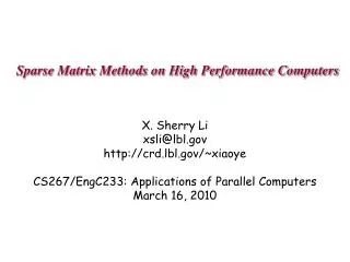
Sparse Direct Solvers on High Performance Computers X. Sherry Li xsli@lbl.gov http://crd.lbl.gov/~xiaoye CS267: Applications of Parallel Computers April 25, 2006
Review of Gaussian Elimination (GE) • Solving a system of linear equations Ax = b • First step of GE: • Repeats GE on C • Results in LU factorization (A = LU) • L lower triangular with unit diagonal, U upper triangular • Then, x is obtained by solving two triangular systems with L and U
Sparse GE • Sparse systems are ubiquitous • Example: A of dimension 105,only 10~100 nonzeros per row • Goal: Store only nonzeros and perform operations only on nonzeros • Fill-in: original zero entry aijbecomes nonzero in L and U Natural order: nonzeros = 233Min. Degree order: nonzeros = 207
nzval 1 c 2 d e 3 k a 4 h b f 5 i l 6 g j 7 rowind 1 3 2 3 4 3 7 1 4 6 2 4 5 6 7 6 5 6 7 colptr 1 3 6 8 11 16 17 20 Compressed Column Storage (CCS) • Also known as Harwell-Boeing format • Store nonzeros columnwise contiguously • 3 arrays: • Storage: NNZ reals, NNZ+N+1 integers • Efficient for columnwise algorithms • Ref: Templates for the Solution of Linear Systems: Building Blocks for Iterative Methods, R. Barrett et al.
Numerical Stability: Need for Pivoting • One step of GE: • If α is small, some entries in B may be lost from addition • Pivoting: swap the current diagonal entry with a larger entry from the other part of the matrix • Goal: prevent from getting too large
Dense versus Sparse GE • Dense GE: Pr A Pc = LU • Pr and Pc are permutations chosen to maintain stability • Partial pivoting suffices in most cases : PrA = LU • Sparse GE: Pr A Pc = LU • Pr and Pc are chosen to maintain stability and preserve sparsity
Algorithmic Issues in Sparse GE • Minimize number of fill-ins, maximize parallelism • Sparsity structure of L & U depends on that of A, which can be changed by row/column permutations (vertex re-labeling of the underlying graph) • Ordering (combinatorial algorithms; NP-complete to find optimum [Yannakis ’83]; use heuristics) • Predict the fill-in positions in L & U • Symbolic factorization (combinatorial algorithms) • Perform factorization and triangular solutions • Numerical algorithms (F.P. operations only on nonzeros) • How and when to pivot ? • Usually dominate the total runtime
Numerical Pivoting • Goal of pivoting is to control element growth in L & U for stability • For sparse factorizations, often relax the pivoting rule to trade with better sparsity and parallelism (e.g., threshold pivoting, static pivoting) • Partial pivoting used in sequential SuperLU (GEPP) • Can force diagonal pivoting (use diagonal threshold) • Hard to implement scalably for sparse factorization • Static pivoting used in SuperLU_DIST (GESP) • Before factor, scale and permute A to maximize diagonal: Pr Dr A Dc = A’ • Pr is found by a weighted bipartite matching algorithm on G(A) • During factor A’ = LU, replace tiny pivots by , without changing data structures for L & U • If needed, use a few steps of iterative refinement to improve the first solution • Quite stable in practice x s x b x x x
4 1 x x 3 x 4 5 2 2 2 1 3 3 4 4 5 5 5 3 Static Pivoting via Weighted Bipartite Matching G(A) A • Maximize the diag. entries: sum, or product (sum of logs) • Hungarian algo. or the like (MC64): O(n*(m+n)*log n) • Auction algo. (more parallel): O(n*m*log(n*C)) • J. Riedy’s dissertation (expected Dec. 2006?) 1 1 row column
i i j k j k 1 1 i i Eliminate 1 j j k k • Undirected graph • After a vertex is eliminated, all its neighbors become a clique • The edges of the clique are the potential fills (upper bound !) 1 i i j j Eliminate 1 k k Structural Gaussian Elimination - Symmetric Case
Minimum Degree Ordering (1/2) • Greedy approach: do the best locally • Best for modest size problems • Hard to parallelize • At each step • Eliminate the vertex with the smallest degree • Update degrees of the neighbors • Straightforward implementation is slow and requires too much memory • Newly added edges are more than eliminated vertices
Minimum Degree Ordering (2/2) • Use quotient graph as a compact representation [George/Liu ’78] • Collection of cliques resulting from the eliminated vertices affects the degree of an uneliminated vertex • Represent each connected component in the eliminated subgraph by a single “supervertex” • Storage required to implement QG model is bounded by size of A • Large body of literature on implementation variants • Tinney/Walker `67, George/Liu `79, Liu `85, Amestoy/Davis/Duff `94, Ashcraft `95, Duff/Reid `95, et al., . .
Nested Dissection Ordering (1/2) • Global graph partitioning approach: top-down, divide-and-conquer • Best for largest problems • Parallel code available: e.g., ParMETIS • Nested dissection [George ’73, Lipton/Rose/Tarjan ’79] • First level • Recurse on A and B • Goal: find the smallest possible separator S at each level • Multilevel schemes [Hendrickson/Leland `94, Karypis/Kumar `95] • Spectral bisection [Simon et al. `90-`95] • Geometric and spectral bisection [Chan/Gilbert/Teng `94] A S B
Ordering for LU (unsymmetric) • Can use a symmetric ordering on a symmetrized matrix . . . • Case of partial pivoting (sequential SuperLU): Use ordering based on ATA • If RTR = ATA and PA = LU, then for any row permutation P, struct(L+U) struct(RT+R) [George/Ng `87] • Making R sparse tends to make L & U sparse . . . • Case of static pivoting (SuperLU_DIST): Use ordering based on AT+A • If RTR = AT+A and A = LU, then struct(L+U) struct(RT+R) • Making R sparse tends to make L & U sparse . . . • Can find better ordering based solely on A, without symmetrization [Amestoy/Li/Ng `03]
Ordering for LU • Still wide open . . . • Simple extension: symmetric ordering using A’+A • Greedy algorithms, graph partitioning, or hybrid • Problem: unsymmetric structure is not respected ! • We developed an unsymmetric variant of “Min Degree” algorithm based solely on A [Amestoy/Li/Ng ’02] (a.k.a. Markowitz scheme)
c1 c2 c3 c1 c2 c3 1 1 r1 r1 Eliminate 1 Eliminate 1 r2 r2 • Bipartite graph • After a vertex is eliminated, all the row & column vertices adjacent to • it become fully connected – “bi-clique” (assuming diagonal pivot) • The edges of the bi-clique are the potential fills (upper bound!) r1 r1 1 c1 1 c1 c2 c2 r2 r2 c3 c3 Structural Gaussian Elimination - Unsymmetric Case
Results of Markowitz Ordering • Extend the QG model to bipartite quotient graph • Same asymptotic complexity as symmetric MD • Space is bounded by 2*(m + n) • Time is bounded by O(n * m) • For 50+ unsym. matrices, compared with MD on A’+A: • Reduction in fill: average 0.88, best 0.38 • Reduction in f.p. operations: average0.77, best 0.01 • How about graph partitioning? (open problem) • Use directed graph
High Performance Issues: Reduce Cost of Memory Access & Communication • Blocking to increase number of floating-point operations performed for each memory access • Aggregate small messages into one larger message • Reduce cost due to latency • Well done in LAPACK, ScaLAPACK • Dense and banded matrices • Adopted in the new generation sparse software • Performance much more sensitive to latency in sparse case
Benefits of Supernodes: Permit use of Level 3 BLAS (e.g., matrix-matrix mult.) Reduce inefficient indirect addressing. Reduce symbolic time by traversing supernodal graph. Exploit dense submatrices in L & U factors Blocking in Sparse GE
Speedup Over Un-blocked Code • Matrices sorted in increasing #Flops/nonzeros • Up to 40% of machine peak on large sparse matrices on IBM RS6000/590, MIPS R8000, 25% on Alpha 21164
Parallel Task Scheduling for SMPs (in SuperLU_MT) • Elimination tree exhibits parallelism and dependencies Shared task queue initialized by leaves While ( there are more panels ) do panel := GetTask( queue ) (1) panel_symbolic_factor( panel ) Skip all BUSY descendant supernodes (2) panel_numeric_factor( panel ) Perform updates from all DONE Wait for BUSY supernodes to become DONE (3) inner_factor( panel ) End while • Up to 25-30% machine peak, 20 processors, Cray C90/J90, SGI Origin • Model speedup by critical path: 10~100 • [Demmel/Gilbert/Li ’99]
Parallelism from Separator Tree • Graph partitioning type of ordering
Parallel Symbolic Factorization [Grigori/Demmel/Li ‘06] • Parallel ordering with ParMETIS on G(A’+A) • Separator tree (binary) to guide computation • Each step: one row of U, one column of L • Within each separator: 1D block cyclic distribution • Send necessary contribution to parent processor • Results: • Reasonable speedup: up to 6x • 5x reduction in maximum per-processor memory needs • Need improve memory balance
Matrix Distribution on Large Distributed-memory Machine • 2D block cyclic recommended for many linear algebra algorithms • Better load balance, less communication, and BLAS-3 1D blocked 1D cyclic 1D block cyclic 2D block cyclic
2D Block Cyclic Layout for Sparse L and U (in SuperLU_DIST) • Better for GE scalability, load balance
Scalability and Isoefficiency Analysis • Model problem: matrix from 11 pt Laplacian on k x k x k (3D) mesh; Nested dissection ordering • N = k3 • Factor nonzeros : O(N4/3) • Number of floating-point operations : O(N2) • Total communication overhead : O(N4/3 P) (assuming P processors arranged as grid) • Isoefficiency function: Maintain constant efficiency if Work increases proportionally with Overhead: This is equivalent to: • (Memory-processor relation) • Parallel efficiency can be kept constant if the memory-per-processor is constant, same as dense LU in ScaLPAPACK • (Work-processor relation)
Scalability • 3D KxKxK cubic grids, scale N2 = K6 with P for constant work per processor • Achieved 12.5 and 21.2 Gflops on 128 processors • Performance sensitive to communication latency • Cray T3E latency: 3 microseconds ( ~ 2702 flops) • IBM SP latency: 8 microseconds ( ~ 11940 flops )
Adoptions of SuperLU • Industrial • FEMLAB • HP Mathematical Library • NAG • Numerical Python • Visual Numerics: IMSL • Academic/Lab: • In other ACTS Tools: PETSc, Hypre • M3D, NIMROD (simulate fusion reactor plasmas) • Omega3P (accelerator design, SLAC) • OpenSees (earthquake simluation, UCB) • DSpice (parallel circuit simulation, SNL) • Trilinos (object-oriented framework encompassing various solvers, SNL) • NIKE (finite element code for structural mechanics, LLNL)
Summary • Important kernel for science and engineering applications, used in practice on a regular basis • Good implementation on high-performance machines needa large set of tools from CS and NLA • Performance more sensitive to latency than dense case • Survey of other sparse direct solvers: “Eigentemplates” book http://crd.lbl.gov/~xiaoye/SuperLU/SparseDirectSurvey.pdf • LLT, LDLT, LU, QR
Open Problems • Much room for optimizing parallel performance • Automatic tuning of blocking parameters • Use of modern programming language to hide latency (e.g., UPC) • Graph partitioning ordering for unsymmetric LU • Scalability of sparse triangular solve • Switch-to-dense • Partitioned inverse • Efficient incomplete factorization (ILU preconditioner) – both sequential and parallel • Optimal complexity sparse factorization (new!) • In the spirit of fast multipole method, but for matrix inversion • J. Xia’s dissertation (expected May 2006)
Model Problem • Discretized system Ax = b from certain PDEs, e.g., 5-point stencil on n x n grid, N = n^2 • Nested dissection ordering gave optimal complexity in exact arithmetic [Hoffman/Martin/Ross] • Factorization cost: O(n^3)
Superfast Factorization: Exploit Low-rank Property • Consider top-level dissection: • S is full • Needs O(n^3) to find u3 • But, off-diagonal blocks of S has low numerical ranks (e.g. 10~15) • U3 can be computed in O(n) flops • Generalizing to multilevel dissection: all diagonal blocks corresp. to the separators have the similar low rank structure • Low rank structures can be represented by hierarchical semi-separable (HSS) matrices [Gu et al.] (… think about SVD) • Factorization complexity … essentially linear • 2D: O(p n^2), p is related to the problem and tolerance (numerical rank) • 3D: O(c(p) n^3), c(p) is a polynomial of p
Results for the Model Problem • Flops and times comparison
Research Issues • Analysis of 3D problems, and complex geometry • Larger tolerance preconditioner (another type of ILU) • If SPD, want all the low rank structures to remain SPD (“Schur-monotonic” talk by M. Gu, Wed, 5/3) • Performance tuning for many small dense matrices (e.g. 10~20) • Switching level in a hybrid solver • Benefits show up only for large enough mesh • Local ordering of unknowns • E.g.: node ordering within a separator affects numerical ranks • Parallel algorithm and implementation
Application 1: Quantum Mechanics • Scattering in a quantum system of three charged particles • Simplest example is ionization of a hydrogen atom by collision with an electron: e- + H H+ + 2e- • Seek the particles’ wave functions represented by the time-independent Schrodinger equation • First solution to this long-standing unsolved problem [Recigno, McCurdy, et al. Science, 24 Dec 1999]
Quantum Mechanics (cont.) • Finite difference leads to complex, unsymmetric systems, very ill-conditioned • Diagonal blocks have the structure of 2D finite difference Laplacian matrices Very sparse: nonzeros per row <= 13 • Off-diagonal block is a diagonal matrix • Between 6 to 24 blocks, each of order between 200K and 350K • Total dimension up to 8.4 M • Too much fill if use direct method . . .
SuperLU_DIST as Preconditioner • SuperLU_DIST as block-diagonal preconditioner for CGS iteration M-1A x = M-1b M = diag(A11, A22, A33, …) • Run multiple SuperLU_DIST simultaneously for diagonal blocks • No pivoting, nor iterative refinement • 12 to 35 CGS iterations @ 1 ~ 2 minute/iteration using 64 IBM SP processors • Total time: 0.5 to a few hours
Complex, unsymmetric N = 2 M, NNZ = 26 M Fill-ins using Metis: 1.3 G (50x fill) Factorization speed 10x speedup (4 to 128 P) Up to 30 Gflops One Block Timings on IBM SP
Application 2: Accelerator Cavity Design • Calculate cavity mode frequencies and field vectors • Solve Maxwell equation in electromagnetic field • Omega3P simulation code developed at SLAC Omega3P model of a 47-cell section of the 206-cell Next Linear Collider accelerator structure Individual cells used in accelerating structure
Finite element methods lead to large sparse generalized eigensystem K x = M x Real symmetric for lossless cavities; Complex symmetric when lossy in cavities Seek interior eigenvalues (tightly clustered) that are relatively small in magnitude Accelerator (cont.)
Accelerator (cont.) • Speed up Lanczos convergence by shift-invert Seek largest eigenvalues, well separated, of the transformed system M (K - M)-1 x = M x = 1 / ( - ) • The Filtering algorithm [Y. Sun] • Inexact shift-invert Lanczos + JOCC (Jacobi Orthogonal Component Correction) • We added exact shift-invert Lanczos (ESIL) • PARPACK for Lanczos • SuperLU_DIST for shifted linear system • No pivoting, nor iterative refinement
DDS47, Linear Elements • Total eigensolver time: N = 1.3 M, NNZ = 20 M
Largest Eigen Problem Solved So Far • DDS47, quadratic elements • N = 7.5 M, NNZ = 304 M • 6 G fill-ins using Metis • 24 processors (8x3) • Factor: 3,347 s • 1 Solve: 61 s • Eigensolver: 9,259 s (~2.5 hrs) • 10 eigenvalues, 1 shift, 55 solves