Download
1 / 58
580 likes | 645 Views
Haplotyping via Perfect Phylogeny - Model, Algorithms, Empirical studies. Dan Gusfield, Ren Hua Chung U.C . Davis Cocoon 2003. Genotypes and Haplotypes. Each individual has two “copies” of each chromosome.

E N D
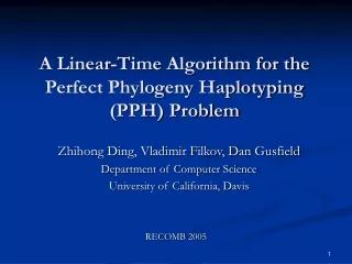
Haplotyping via Perfect Phylogeny - Model, Algorithms, Empirical studies Dan Gusfield, Ren Hua Chung U.C. Davis Cocoon 2003
Genotypes and Haplotypes Each individual has two “copies” of each chromosome. At each site, each chromosome has one of two alleles (states) denoted by 0 and 1 (motivated by SNPs) 0 1 1 1 0 0 1 1 0 1 1 0 1 0 0 1 0 0 Two haplotypes per individual Merge the haplotypes 2 1 2 1 0 0 1 2 0 Genotype for the individual
SNP Data • A SNP is a Single Nucleotide Polymorphism - a site in the genome where two different nucleotides appear with sufficient frequency in the population (say each with 5% frequency or more). • SNP maps have been compiled with a density of about 1 site per 1000. • SNP data is what is mostly collected in populations - it is much cheaper to collect than full sequence data, and focuses on variation in the population, which is what is of interest.
Haplotype Map Project: HAPMAP • NIH lead project ($100M) to find common haplotypes in the Human population. • Used to try to associate genetic-influenced diseases with specific haplotypes, to either find causal haplotypes, or to find the region near causal mutations. • Haplotyping individuals is expensive.
Haplotyping Problem • Biological Problem: For disease association studies, haplotype data is more valuable than genotype data, but haplotype data is hard to collect. Genotype data is easy to collect. • Computational Problem: Given a set of n genotypes, determine the original set of n haplotypepairs that generated the n genotypes. This is hopeless without a genetic model.
The Perfect Phylogeny Model of Haplotype Evolution sites 12345 Ancestral haplotype 00000 1 4 Site mutations on edges 3 00010 2 10100 5 10000 01010 01011 Extant haplotypes at the leaves
The Perfect Phylogeny Model We assume that the evolution of extant haplotypes can be displayed on a rooted, directed tree, with the all-0 haplotype at the root, where each site changes from 0 to 1 on exactly one edge, and each extant haplotype is created by accumulating the changes on a path from the root to a leaf, where that haplotype is displayed. In other words, the extant haplotypes evolved along a perfect phylogeny with all-0 root.
Perfect Phylogeny Haplotype (PPH) Given a set of genotypes S, find an explaining set of haplotypes that fits a perfect phylogeny. sites A haplotype pair explains a genotype if the merge of the haplotypes creates the genotype. Example: The merge of 0 1 and 1 0 explains 2 2. S Genotype matrix
The PPHProblem Given a set of genotypes, find an explaining set of haplotypes that fits a perfect phylogeny
The Haplotype PhylogenyProblem Given a set of genotypes, find an explaining set of haplotypes that fits a perfect phylogeny 00 1 2 b 00 a a b c c 01 01 10 10 10
The Alternative Explanation No tree possible for this explanation
Efficient Solutions to the PPH problem - n genotypes, m sites • Reduction to a graph realization problem (GPPH) - build on Bixby-Wagner or Fushishige solution to graph realization O(nm alpha(nm)) time. • Reduction to graph realization - build on Tutte’s graph realization method O(nm^2) time. • Direct, from scratch combinatorial approach -O(nm^2) Bafna et al. • Berkeley (EHK) approach - specialize the Tutte solution to the PPH problem - O(nm^2) time.
The case of the 1’s • For any row i in S, the set of 1 entries in row i specify the exact set of mutations on the path from the root to the least common ancestor of the two leaves labeled i, in every perfect phylogeny for S. • The order of those 1 entries on the path is also the same in every perfect phylogeny for S, and is easy to determine by “leaf counting”.
In any column c, count two for each 1, and count one for each 2. The total is the number of leaves below mutation c, in every perfect phylogeny for S. So if we know the set of mutations on a path from the root, we know their order as well. Leaf Counting S Count 5 4 2 2 1 1 1
So Assume The columns are sorted by leaf-count, largest to the left.
Similarly In any perfect phylogeny, the edge corresponding to the leftmost 2 in a row must be on a path just after the 1’s for that row.
Simple Conclusions Subtree for row i data sites Root 1 2 3 4 5 6 7 i:0 1 0 1 222 The order is known for the red mutations together with the leftmost blue mutation. 2 4 5
But what to do with the remaining blue entries (2’s) in a row?
More Simple Tools • For any row i in S, and any column c, if S(i,c) is 2, then in every perfect phylogeny for S, the path between the two leaves labeled i, must contain the edge with mutation c. Further, every mutation c on the path between the two i leaves must be from such a column c.
From Row Data to Tree Constraints Subtree for row i data sites Root 1 2 3 4 5 6 7 i:0 1 0 1 222 2 4 Edges 5, 6 and 7 must be on the blue path, and 5 is already known to follow 4, but we don’t where to put 6 and 7. 5 i i
The Graph Theoretic Problem Given a genotype matrix S with n sites, and a red-blue subgraph for each row i, create a directed tree T where each integer from 1 to n labels exactly one edge, so that each subgraph is contained in T. i i
Powerfull Tool: Graph Realization • Let Rn be the integers 1 to n, and let P be an unordered subset of Rn. P is called a path set. • A tree T with n edges, where each is labeled with a unique integer of Rn, realizes P if there is a contiguous path in T labeled with the integers of P and no others. • Given a family P1, P2, P3…Pk of path sets, tree T realizes the family if it realizes each Pi. • The graph realization problem generalizes the consecutive ones problem, where T is a path.
Graph Realization Example 5 P1: 1, 5, 8 P2: 2, 4 P3: 1, 2, 5, 6 P4: 3, 6, 8 P5: 1, 5, 6, 7 1 8 6 2 4 3 7 Realizing Tree T
Graph Realization Polynomial time (almost linear-time) algorithms exist for the graph realization problem – Whitney, Tutte, Cunningham, Edmonds, Bixby, Wagner, Gavril, Tamari, Fushishige, Lofgren 1930’s - 1980’s The algorithms are not simple; none implemented before 2002.
Reducing PPH to graph realization We solve any instance of the PPH problem by creating appropriate path sets, so that a solution to the resulting graph realization problem leads to a solution to the PPH problem instance. The key issue: How to encode the needed subgraph for each row, and glue them together at the root.
From Row Data to Tree Constraints Subtree for row i data sites Root 1 2 3 4 5 6 7 i:0 1 0 1 222 2 4 Edges 5, 6 and 7 must be on the blue path, and 5 is already known to follow 4. 5 i i
Encoding a Red-Blue directed path 2 P1: U, 2 P2: U, 2, 4 P3: 2, 4 P4: 2, 4, 5 P5: 4, 5 U 4 2 5 4 forced In T 5 U is a glue edge used to glue together the directed paths from the different rows.
Now add a path set for the blues in row i. sites Root 1 2 3 4 5 6 7 i:0 1 0 1 222 2 4 5 P: 5, 6, 7 i i
That’s the Reduction The resulting path-sets encode everything that is known about row i in the input. The family of path-sets are input to the graph- realization problem, and every solution to the that graph-realization problem specifies a solution to the PPH problem, and conversely. But how is graph realization solved?
Tutte’s Algorithm for Graph Realization, given a partial solution T. • Pick an unpicked edge e. • Determine any other edges that must be on one particular side of e or the other. • Determine any pair of edges that must be on opposite sides of e. Form a graph G with an edge between any such pair - test if bipartite. If so, assign one side of G to one side of e, and the other side of G to the other side of e. • Apply the decisions, modifying T, and recurse.
GPPH: An implementation of a variation of Tutte’s algorithm • The variation is due to Gavril and Tamari. • About 1000 lines of C to do the reduction explicitly, and about 4000 lines of C to implement the fully general graph-realization algorithm. • O(nm^2) time. • We did not (yet) implement an O(nm alpha(nm)) method for graph realization.
HPPH (BPPH) EHK Method • Eskin, Halperin, Karp method can be viewed as specializing the Tutte method to the PPH problem - takes advantage of the fact that the PPH solution is a directed, rooted tree, and with leaf-counting, ordering information is known. Other local rules determine whether an edge must be on one side (below) e, and whether two edges can be deduced to be on opposite sides of e. • O(nm^2) time.
The DPPH Method • Bafna et al. O(nm^2) time • Based on deeper combinatorial observations about the PPH problem. • A matrix-centric approach (rather than tree-centric), although a graph is used in the algorithm. First, we need to understand why some sets of haplotypes have a perfect phylogeny, and some do not.
When does a set of haplotypes fit a perfect phylogeny? Classic NASC: Arrange the haplotypes in a matrix, two haplotypes for each individual. Then (with no duplicate columns), the haplotypes fit a unique perfect phylogeny if and only if no two columns contain all three pairs: 0,1 and 1,0 and 1,1 This is the 3-Gamete Test
The Alternative Explanation No tree possible for this explanation
The Tree Explanation Again 0 0 1 2 b 0 0 a b a c c 0 1 0 1
PPH: The Combinatorial Problem Input: A ternary matrix (0,1,2) M with 2N rows partitioned into N pairs of rows, where the two rows in each pair are identical. Def: If a pair of rows (r,r’) in the partition have entry values of 2 in a column j then positions (r,j) and (r’,j) are called Mates.
Output: A binary matrix M’ created from M by replacing each 2 in M with either 0 or 1, such that A position is assigned 0 if and only if its Mate is assigned 1. b) M’ passes the 3-Gamete Test, i.e., does not contain a 3x2 submatrix (after row and column permutations) with all three combinations 0,1; 1,0; and 1,1
Initial Observations If two columns of M contain the following rows 2 0 2 0 mates 0 2 0 2 mates then M’ will contain a row with 1 0 and a row with 0 1 in those columns. This is a forced expansion.
Initial Observations Similarly, if two columns of M contain the mates 2 1 2 1 then M’ will contain a row with 1 1 in those columns. This is a forced expansion.
If a forced expansion of two columns creates 0 1 in those columns, then any 2 2 1 0 2 2 in those columns must be set to be 0 1 1 0 We say that two columns are forced out-of-phase. If a forced expansion of two columns creates 1 1 in those columns, then any 2 2 2 2 in those columns must be set to be 1 1 0 0 We say that two columns are forced in-phase.
1 2 3 a Example: a Columns 1 and 2, and 1 and 3 are forced in-phase. Columns 2 and 3 are forced out-of-phase. b b c c d d e e
Overview of Bafna et al. algorithm First, represent the forced phase relationships, and the needed decisions, in a graph G.
7 1 Graph G Each node represents a column in M, and each edge indicates that the pair of columns has a row with 2’s in both columns. The algorithm builds this graph, and then checks whether any pair of nodes is forced in or out of phase. 6 3 4 2 5
7 1 Graph Gc Each Red edge indicates that the columns are forced in-phase. Each Blue edge indicates that the columns are forced out-of-phase. 6 3 4 2 Let Gf be the subgraph of Gc defined by the red and blue edges. 5
7 1 Graph Gf has three connected components. 6 3 4 2 5
The Central Theorem There is a solution to the PPH problem for M if and only if there is a coloring of the dashed edges of Gc with the following property: For any triangle (i,j,k) in Gc, where there is one row containing 2’s in all three columns i,j and k (any triangle containing at least one dashed edge will be of this type), the coloring makes either 0 or 2 of the edges blue (out-of-phase). Nice, but how do we find such a coloring?
7 1 Triangle Rule Graph Gf Theorem 1: If there are any dashed edges whose ends are in the same connected component of Gf, at least one edge is in a triangle where the other edges are not dashed, and in every PPH solution, it must be colored so that the triangle has an even number of Blue (out of Phase) edges. This is an “inferred” coloring. 6 3 4 2 5
7 1 6 3 4 2 5