How might climate change affect this story?

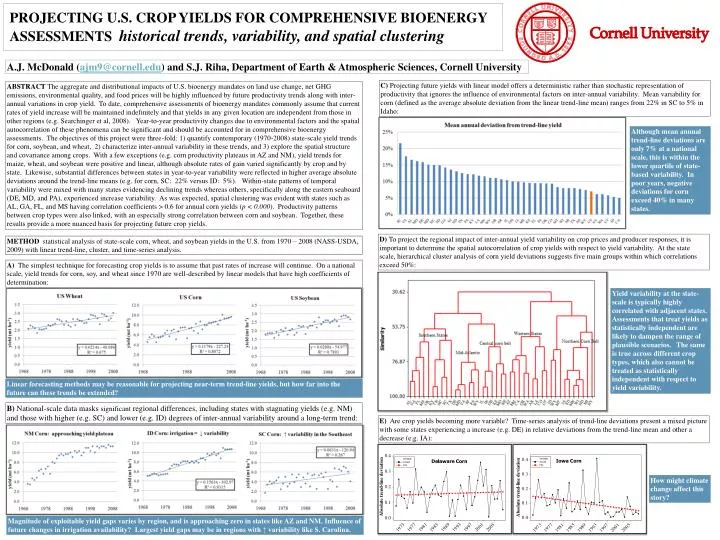
1. A.J. McDonald (ajm9@cornell.edu) and S.J. Riha, Department of Earth & Atmospheric Sciences, Cornell University C) Projecting future yields with linear model offers a deterministic rather than stochastic representation of productivity that ignores the influence of environmental factors on inter-annual variability. Mean variability for corn (defined as the average absolute deviation from the linear trend-line mean) ranges from 22% in SC to 5% in Idaho: ABSTRACT The aggregate and distributional impacts of U.S. bioenergy mandates on land use change, net GHG emissions, environmental quality, and food prices will be highly influenced by future productivity trends along with inter-annual variations in crop yield. To date, comprehensive assessments of bioenergy mandates commonly assume that current rates of yield increase will be maintained indefinitely and that yields in any given location are independent from those in other regions (e.g. Searchinger et al, 2008). Year-to-year productivity changes due to environmental factors and the spatial autocorrelation of these phenomena can be significant and should be accounted for in comprehensive bioenergy assessments. The objectives of this project were three-fold: 1) quantify contemporary (1970-2008) state-scale yield trends for corn, soybean, and wheat, 2) characterize inter-annual variability in these trends, and 3) explore the spatial structure and covariance among crops. With a few exceptions (e.g. corn productivity plateaus in AZ and NM), yield trends for maize, wheat, and soybean were positive and linear, although absolute rates of gain varied significantly by crop and by state. Likewise, substantial differences between states in year-to-year variability were reflected in higher average absolute deviations around the trend-line means (e.g. for corn, SC: 22% versus ID: 5%). Within-state patterns of temporal variability were mixed with many states evidencing declining trends whereas others, specifically along the eastern seaboard (DE, MD, and PA), experienced increase variability. As was expected, spatial clustering was evident with states such as AL, GA, FL, and MS having correlation coefficients > 0.6 for annual corn yields (p < 0.000). Productivity patterns between crop types were also linked, with an especially strong correlation between corn and soybean. Together, these results provide a more nuanced basis for projecting future crop yields. Although mean annual trend-line deviations are only 7% at a national scale, this is within the lower quartile of state-based variability. In poor years, negative deviations for corn exceed 40% in many states. PROJECTING U.S. CROP YIELDS FOR COMPREHENSIVE BIOENERGY ASSESSMENTS historical trends, variability, and spatial clustering D) To project the regional impact of inter-annual yield variability on crop prices and producer responses, it is important to determine the spatial autocorrelation of crop yields with respect to yield variability. At the state scale, hierarchical cluster analysis of corn yield deviations suggests five main groups within which correlations exceed 50%: METHOD statistical analysis of state-scale corn, wheat, and soybean yields in the U.S. from 1970 – 2008 (NASS-USDA, 2009) with linear trend-line, cluster, and time-series analysis. A) The simplest technique for forecasting crop yields is to assume that past rates of increase will continue. On a national scale, yield trends for corn, soy, and wheat since 1970 are well-described by linear models that have high coefficients of determination: Yield variability at the state-scale is typically highly correlated with adjacent states. Assessments that treat yields as statistically independent are likely to dampen the range of plausible scenarios. The same is true across different crop types, which also cannot be treated as statistically independent with respect to yield variability. Linear forecasting methods may be reasonable for projecting near-term trend-line yields, but how far into the future can these trends be extended? B) National-scale data masks significant regional differences, including states with stagnating yields (e.g. NM) and those with higher (e.g. SC) and lower (e.g. ID) degrees of inter-annual variability around a long-term trend: E) Are crop yields becoming more variable? Time-series analysis of trend-line deviations present a mixed picture with some states experiencing a increase (e.g. DE) in relative deviations from the trend-line mean and other a decrease (e.g. IA): How might climate change affect this story? Magnitude of exploitable yield gaps varies by region, and is approaching zero in states like AZ and NM. Influence of future changes in irrigation availability? Largest yield gaps may be in regions with ↑ variability like S. Carolina.