Download
1 / 171
1.73k likes | 2.2k Views
Computational Chemistry. G. H. CHEN Department of Chemistry University of Hong Kong. Beginning of Computational Chemistry. In 1929, Dirac declared, “The underlying physical laws necessary for the mathematical theory of ...the whole of chemistry are thus completely know, and

E N D
Computational Chemistry G. H. CHEN Department of Chemistry University of Hong Kong
Beginning of Computational Chemistry In 1929, Dirac declared, “The underlying physical laws necessary for the mathematical theory of ...the whole of chemistry are thus completely know, and the difficulty is only that the exact application of these laws leads to equations much too complicated to be soluble.” Dirac
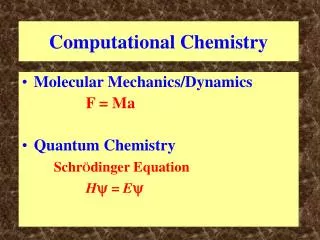
Computational Chemistry Quantum Chemistry Molecular Mechanics SchrÖdinger Equation F = M a
Nobel Prizes for Computational Chemsitry Mulliken,1966 Fukui, 1981 Hoffmann, 1981 Pople, 1998 Kohn, 1998
Computational Chemistry Industry Company Software Gaussian Inc. Gaussian 94, Gaussian 98 Schrödinger Inc. Jaguar Wavefunction Spartan Q-Chem Q-Chem Accelrys InsightII, Cerius2 HyperCube HyperChem Celera Genomics (Dr. Craig Venter, formal Prof., SUNY, Baffalo; 98-01) Applications: material discovery, drug design & research
Calculated STM Image of a Carbon Nanotube (Rubio, 1999) STM Image of Carbon Nanotubes (Wildoer et. al., 1998)
Computer Simulations (Saito, Dresselhaus, Louie et. al., 1992) Carbon Nanotubes (n,m): Conductor, if n-m = 3I I=0,±1,±2,±3,…;or Semiconductor, if n-m 3I Metallic Carbon Nanotubes: Conducting Wires Semiconducting Nanotubes: Transistors Molecular-scale circuits ! 1 nm transistor! 30 nm transistor! 0.13 µm transistor!
Experimental Confirmations: Lieber et. al. 1993; Dravid et. al., 1993; Iijima et. al. 1993; Smalley et. al. 1998; Haddon et. al. 1998; Liu et. al. 1999 Wildoer, Venema, Rinzler, Smalley, Dekker, Nature 391, 59 (1998)
RL 7.39 kΩ L 16.6 pH Rc 6.45 kΩ (0.5g0-1) C 0.073 aF g0=2e2/h L ~ ~ ≈ 18.8 pH Yam, Mo, Wang, Li, Chen, Zheng, Goddard (2008)
Microelectromechanical Systems (MEMS) Micro-Electro-Mechanical Systems (MEMS) is the integration of mechanical elements, sensors, actuators, and electronics on a common silicon substrate through microfabrication technology. While the electronics are fabricated using integrated circuit (IC) process sequences (e.g., CMOS, Bipolar, or BICMOS processes), the micromechanical components are fabricated using compatible "micromachining" processes that selectively etch away parts of the silicon wafer or add new structural layers to form the mechanical and electromechanical devices. Nanoelectromechanical Systems (NEMS) K.E. Drexler, Nanosystems: Molecular Machinery, anufacturing and Computation (Wiley, New York, 1992).
Large Gear Drives Small Gear G. Hong et. al., 1999
Nano-oscillators Nanoscopic Electromechanical Device (NEMS) Zhao, Ma, Chen & Jiang, Phys. Rev. Lett. 2003
Computer-Aided Drug Design Human Genome Project GENOMICS Drug Discovery
ALDOSE REDUCTASE Diabetic Complications Diabetes Sorbitol Glucose
Design of Aldose Reductase Inhibitors Inhibitor Aldose Reductase Hu, Chen & Chau, J. Mol. Graph. Mod. 24 (2006)
Prediction Results using AutoDock LogIC50: 0.77,1.1 LogIC50: -1.87,4.05 LogIC50: -2.77,4.14 LogIC50: 0.68,0.88 Hu, Chen & Chau, J. Mol. Graph. Mod. 24 (2006)
Computer-aided drug design Chemical Synthesis Screening using in vitro assay Animal Tests Clinical Trials
Quantum Chemistry G. H. Chen Department of Chemistry University of Hong Kong
Contributors: Hartree, Fock, Slater, Hund, Mulliken, Lennard-Jones, Heitler, London, Brillouin, Koopmans, Pople, Kohn Application: Chemistry, Condensed Matter Physics, Molecular Biology, Materials Science, Drug Discovery
Emphasis Hartree-Fock method Concepts Hands-on experience Text Book “Quantum Chemistry”, 4th Ed. Ira N. Levine http://yangtze.hku.hk/lecture/chem3504-3.ppt
Quantum Chemistry Methods • Ab initio molecular orbital methods • Semiempirical molecular orbital methods • Density functional method
SchrÖdinger Equation Hy = Ey Wavefunction Hamiltonian H = (-h2/2ma)2 - (h2/2me)ii2 + ZaZbe2/rab - i Zae2/ria + ije2/rij Energy
Contents 1. Variation Method 2. Hartree-Fock Self-Consistent Field Method 3. Beyond Hartree-Fock 4. Perturbation Theory 5. Molecular Dynamics
The Variation Method The variation theorem Consider a system whose Hamiltonian operator H is time independent and whose lowest-energy eigenvalue is E1. If f is any normalized, well- behaved function that satisfies the boundary conditions of the problem, then f* Hf dt >E1
Proof: Expand f in the basis set { yk} f = kakyk where {ak} are coefficients Hyk = Ekyk then f* Hf dt = kjak* aj Ej dkj = k | ak|2Ek> E 1k | ak|2 = E1 Since is normalized, f*f dt = k | ak|2 = 1
i. f : trial function is used to evaluate the upper limit of ground state energy E1 ii. f= ground state wave function, f* Hf dt = E1 iii. optimize paramemters in f by minimizing f* Hf dt / f* f dt
Application to a particle in a box of infinite depth l 0 Requirements for the trial wave function: i. zero at boundary; ii. smoothness a maximum in the center. Trial wave function: f = x (l - x)
* H dx = -(h2/82m) (lx-x2) d2(lx-x2)/dx2 dx = h2/(42m) (x2 - lx)dx = h2l3/(242m) * dx = x2 (l-x)2 dx = l5/30 E = 5h2/(42l2m) h2/(8ml2) = E1
Variational Method (1) Construct a wave function (c1,c2,,cm) (2) Calculate the energy of : E E(c1,c2,,cm) (3) Choose {cj*} (i=1,2,,m) so that Eis minimum
Example: one-dimensional harmonic oscillator Potential: V(x) = (1/2) kx2 = (1/2) m2x2 = 22m2x2 Trial wave function for the ground state: (x) = exp(-cx2) * H dx = -(h2/82m) exp(-cx2) d2[exp(-cx2)]/dx2 dx + 22m2 x2 exp(-2cx2) dx = (h2/42m) (c/8)1/2 + 2m2 (/8c3)1/2 * dx = exp(-2cx2) dx = (/2)1/2 c-1/2 E= W = (h2/82m)c + (2/2)m2/c
To minimize W, 0 = dW/dc = h2/82m - (2/2)m2c-2 c = 22m/h W= (1/2) h
Extension of Variation Method . . . E3y3 E2y2 E1y1 For a wave function f which is orthogonal to the ground state wave function y1, i.e. dtf*y1 = 0 Ef = dtf*Hf / dtf*f>E2 the first excited state energy
The trial wave function f: dtf*y1 = 0 f = k=1 akyk dtf*y1 = |a1|2 = 0 Ef = dtf*Hf / dtf*f = k=2|ak|2Ek / k=2|ak|2 >k=2|ak|2E2 / k=2|ak|2 = E2
Application to H2+ e + + y1 y2 f = c1y1 + c2y2 W = f*H f dt / f*f dt = (c12H11 + 2c1 c2H12+ c22H22 ) / (c12 + 2c1 c2S + c22 ) W (c12 + 2c1 c2S + c22) = c12H11 + 2c1 c2H12+ c22H22
Partial derivative with respect to c1(W/c1 = 0) : W (c1 + S c2) = c1H11 + c2H12 Partial derivative with respect to c2(W/c2 = 0) : W (S c1 + c2) = c1H12 + c2H22 (H11 - W) c1 + (H12 - S W) c2 = 0 (H12 - S W) c1 + (H22 -W) c2 = 0
To have nontrivial solution: H11 - W H12 - S W H12 - S W H22 -W For H2+,H11 = H22; H12 < 0. Ground State: Eg = W1 = (H11+H12) / (1+S) f1= (y1+y2) / 2(1+S)1/2 Excited State: Ee = W2 = (H11-H12) / (1-S) f2= (y1-y2) / 2(1-S)1/2 = 0 bonding orbital Anti-bonding orbital
Results: De = 1.76 eV, Re = 1.32 A Exact: De = 2.79 eV, Re = 1.06 A 1 eV = 23.0605 kcal / mol
2p 1s Further Improvements H p-1/2exp(-r) He+ 23/2p-1/2exp(-2r) Optimization of 1s orbitals Trial wave function: k3/2p-1/2exp(-kr) Eg = W1(k,R) at each R, choose kso thatW1/k = 0 Results: De = 2.36 eV, Re = 1.06 A Resutls: De = 2.73 eV, Re = 1.06 A Inclusion of other atomic orbitals
a11x1 + a12x2 = b1 a21x1 + a22x2 = b2 (a11a22-a12a21) x1 = b1a22-b2a12 (a11a22-a12a21) x2 = b2a11-b1a21 Linear Equations 1. two linear equations for two unknown, x1 and x2
Introducing determinant: a11 a12 = a11a22-a12a21 a21 a22 a11 a12b1 a12 x1 = a21 a22 b2 a22 a11 a12a11 b1 x2 = a21 a22a21 b2
Our case: b1 = b2 = 0, homogeneous 1. trivial solution: x1 = x2 = 0 2. nontrivial solution: a11 a12 = 0 a21 a22 n linear equations for n unknown variables a11x1 + a12x2 + ... + a1nxn= b1 a21x1 + a22x2 + ... + a2nxn= b2 ............................................ an1x1 + an2x2 + ... + annxn= bn
a11 a12 ... a1,k-1 b1 a1,k+1 ... a1n a21 a22 ... a2,k-1 b2 a2,k+1 ... a2n det(aij) xk= . . ... . . . ... . an1 an2 ... an,k-1 b2 an,k+1 ... ann where, a11 a12 ... a1n a21 a22 ... a2n det(aij) = . . ... . an1 an2 ... ann
inhomogeneous case: bk = 0 for at least one k a11 a12 ... a1,k-1 b1 a1,k+1 ... a1n a21 a22 ... a2,k-1 b2 a2,k+1 ... a2n . . ... . . . ... . an1 an2 ... an,k-1 b2 an,k+1 ... ann xk = det(aij)
homogeneous case: bk = 0, k = 1, 2, ... , n (a) travial case: xk = 0, k = 1, 2, ... , n (b) nontravial case: det(aij) = 0 For a n-th order determinant, n det(aij) = alk Clk l=1 where, Clk is called cofactor