Download
1 / 46
490 likes | 669 Views
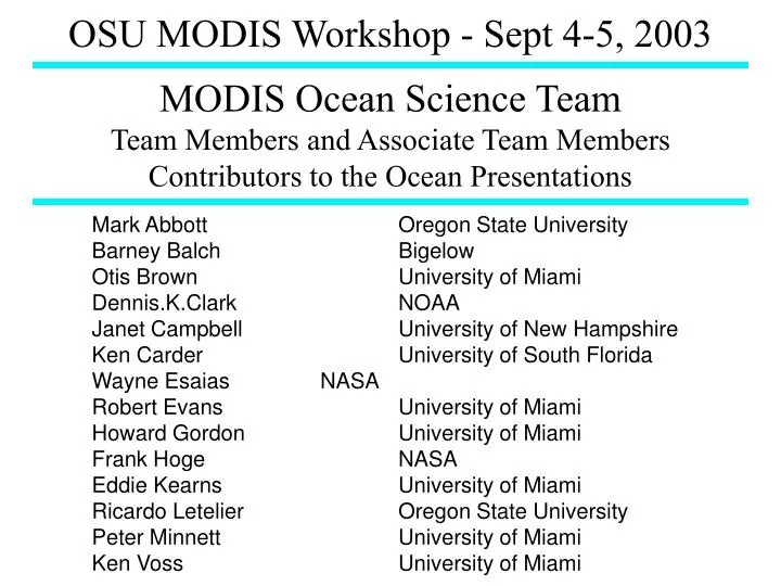
OSU MODIS Workshop - Sept 4-5, 2003. MODIS Ocean Science Team Team Members and Associate Team Members Contributors to the Ocean Presentations. Mark Abbott Oregon State University Barney Balch Bigelow Otis Brown University of Miami Dennis.K.Clark NOAA

E N D
OSU MODIS Workshop - Sept 4-5, 2003 MODIS Ocean Science TeamTeam Members and Associate Team MembersContributors to the Ocean Presentations Mark Abbott Oregon State University Barney Balch Bigelow Otis Brown University of Miami Dennis.K.Clark NOAA Janet Campbell University of New Hampshire Ken Carder University of South Florida Wayne Esaias NASA Robert Evans University of Miami Howard Gordon University of Miami Frank Hoge NASA Eddie Kearns University of Miami Ricardo Letelier Oregon State University Peter Minnett University of Miami Ken Voss University of Miami
Ocean Talk Outline • Thursday • Ocean products Part 1 • MODIS overview (Ocean Team) • Part 2 • Ocean color atmospheric correction (Howard Gordon, Ken Voss, Bob Evans) • nLw calibration, validation (Ed Kearns, Bob Evans, Dennis Clark) • Part 3 • MODIS Chlorophyll product comparison (Dennis Clark, Ken Carder, Janet Campbell) • Examples MODIS • Friday • Part 4 • IR band atmospheric correction (Bob Evans, Peter Minnett, Otis Brown) • SST calibration, validation (Ed Kearns, Bob Evans)
TERRA MODIS NIGHTTIME 4mm SST MAY 2001 V 3.3.1 -2 5 10 15 20 25 30 35 Co MODIS/OCEAN GROUP GSFC, RSMAS
MODIS Instrument Considerations • MODIS algorithms are based on heritage instruments. • How does the MODIS instrument and MODIS orbit impact heritage processing algorithms?
MODIS Comparison to AVHRR, SeaWiFS • 12 bit digitization vs 10 bit -> improved precision • Lower noise detectors -> subtle features better resolved • Global 1 km data stream vs 4km -> larger data sets but spatial features bettwer resolved • Additional spectral channels -> improved and additional product algorithms, better quality determination • Equatorial crossing time -> significant impact on atmospheric correction • Shared calibration sources: optical - MOBY buoy, infrared - MAERI interferometer, buoys
MODIS-AVHRR-SeaWiFS Heritage Instrument Comparison AVHRR Pathfinder SST Nov 1, 2000-306 Night (24 hours) MODIS Thermal SST SeaWiFS Chl-Oc4v4 Nov 1, 2000 Weekly Composite MODIS Chl-MODIS
Characteristics of MODIS IR Focal Planes SST Product Input Bands MODIS has 4 focal planes, each band with 10 - 1km detectors: 2 for visible 2 for IR
Angle of Incidence changes pixel by pixel with Paddle wheel scan mirror MODIS Scan Mirror Angles of Incidence(Earth View: 10.5 to 65.5) Principal Scan Angles(Earth View: -55 to 55 )
Ocean Color Radiances measured by the MODerate resolution Imaging Spectroradiometer (MODIS). R. H. Evans, E. J. Kearns, H. R. Gordon K. Voss, D. Clark & Warner Baringer, Jim Brown, Kay Kilpatrick, Sue Walsh. Meteorology and Physical Oceanography Rosenstiel School of Marine and Atmospheric Science University of Miami MODIS Meeting July 23, 2002
Ocean Color Outline • Atmospheric Correction for ocean color • Impact of MODIS on Atmospheric Correction • Calibration/Validation of MODIS water leaving radiance • MODIS Chlorophyll products
Ocean-Atmosphere SpectrumWater Leaving Radiance Retrieval Challenge MODIS - : At satellite radiance : Rayleigh removed radiance Water leaving radiance: Lw
Gaseous AbsorptionTransparency Windows MODIS SeaWiFS Wavebands 443 488 531 551 MODIS 667 678 749 869 412 443 490 510 555 SeaWiFS667 765 865
Atmospheric Correction Equationt = r + (a + ra) + twc + tg + t w* w is the quantity we wish to retrieve at each wavelength. * g is Sun glint, the direct + diffuse reflectance of the solar radiance from the sea surface. This effect for SeaWiFS is minimized by tilting the sensor. MODIS does not tilt and the sun glint must be removed, depends on vector winds and polarization. * wc is the contribution due to "white"-capping, estimated from statistical relationship with wind speed. * ris the contribution due to molecular (Rayleigh) scattering, which can be accurately modeled. MODIS requires accurate measurement of change in mirror reflectivity with angle of incidence, depends on polarization, winds, atmospheric pressure* a + ra is the contribution due to aerosol and Rayleigh-aerosol scattering, estimated in NIR from measured radiances and extrapolated to visible using aerosol models.* t is the total reflectance measured at the satellite
MODIS - SeaWiFS Atmospheric Correction Differences • Glint - Spectral diffuse glint term, modified Cox-Munk distribution with spectral weighting, must be removed for MODIS (non-tilting), SeaWiFS minimizes glint by tilting • Rayleigh - Polarization varies with satellite and solar zenith angles, MODIS mirror angle of incidence (AOI) affects reflectivity, SeaWiFS has constant AOI mirror • Multiple (10) detectors per spectral band - Affects Rayleigh, especially near nadir, SeaWiFS 1 detector/band • Equatorial crossing time - SeaWiFS noon, MODIS Terra 1030, Aqua 1330. Effects sun glint, bi-directional reflectance
Atmospheric correction enhancements for MODIS • Instruments effects - detector and mirror side banding • Polarization • Sun-glint • Sun-satellite-observation point viewing geometry, overpass time and BRDF -bidirectional reflectance
Southeastern North America nLw 412nm November 1, 2000 Examples of detector and mirror side banding before correction
Northeastern Gulf of Mexico nLw 412 nm November 1, 2000 Mirror Side Banding Detector Striping Scan Line Pixel Number Pixel Number
Correction reduces mirror and detector effects by a factor of 5 Terra Mirror Side Cross-scan vs time gain 412 nm uncorrected 412 nm corrected
Inter-Detector gain adjustments • Correction to reduce detector to detector bias. • Plot of the at-launch relative response of each of the 10 detectors. • A general increasing linear response from detector 1 to detector 10 on the order of ~1% is present in all bands. The black line represents the inter-detector response after gains were adjusted by normalizing response to detector 5 and filtering La.
Atmospheric correction enhancements for MODIS • Instruments effects - detector and mirror side banding • Polarization • Sun-glint • Sun-satellite-observation point viewing geometry, overpass time and BRDF -bidirectional reflectance
Degree of polarization of at sensor total Radiance, Lt Cross scan polarization varies with season and latitude from near 0 to 65% Dec 4, 2000 (solstice) Apr 8, 2001 (equinox) June 10, 2001 (solstice)
Impact of Polarization and cross-scan correction on 412 nm nLw Corrected East/west transition between adjacent orbits not smooth for non-polarization corrected orbits Uncorrected June 412 pol Dec 412 pol Dec 412 nopol June 412 nopol
Atmospheric correction enhancements for MODIS • Instruments effects - detector and mirror side banding • Polarization • Sun-glint • Sun-satellite-observation point viewing geometry, overpass time and BRDF -bidirectional reflectance
Sun glint correction Sun glint influences large portions of the image. Several approaches to correcting the glint problem were investigated. Shape of sun glint determined from Cox-Munk distribution, wind speed dependent. a) We assumed sun glint was direct, include only Rayleigh scattering b) Added an aerosol component to the sun glint. Result: improved Lw retrievals in regions of sun glint contamination with reasonable spectral behavior. c) Include polarization. Sun glint correction currently a workable approximation but is limited both by differences in shape between real sun glint spatial distribution and the shape provided by Cox-Munk and by the accuracy of the NCEP wind fields.
Glint Corrected La 865nm Note ‘wind-wave-current interaction. Glint suppressed in Gulf Stream region Uncorrected La 865nm Yellow - red region glint contaminated (Lg> 5*La). > 70% of swath affected. Corrected La 865nm Sun glint removed La865nm.
Atmospheric correction enhancements for MODIS • Instruments effects - detector and mirror side banding • Polarization • Sun-glint • Sun-satellite-observation point viewing geometry, overpass time and BRDF -bidirectional reflectance
Radiance distributionvs. azimuth and solar zenith angles (Ken Voss)Scan line geometry, variation with Latitude, 0° to 80°N MODIS SeaWiFS Black intrusions mark orientation of Sun. Black line irepresents orbit track Satellite scan changes from near parallel to perpendicular along orbit track Satellite scan more symmetric and perpendicular to orbit track
BRDF Effects on apparent CHL ConcentrationCross-scan variation at selected latitudes MODIS SeaWiFS
Calibration Approach • Use at surface nLw, atmospheric and surface reflectance corrected • Validation site for in situ reference is MOBY @ Hawaii, more extensive validation for other regions will require completion of reprocessing (use of SIMBIOS reference data) • Cross-scan: Referenced to pixel 500, minimum of sun glint • Detector Balance: Referenced to detector 5, low noise, center of detector array • Mirror side Balance: reference to side 1 • Remove time trends: Compare modal peak for area surrounding MOBY to MOBY, high temporal density, not dependent on cloud free conditions • Calibration: Adjust MOBY-MODIS single pixel match-ups to remove bias
MOBY Instrumentand spectralTime Series of MODIS ocean color bands
nLw Modal Terra MODIS-Moby Time Series Modal time series of area around Hawaii used to remove time trends in MODIS calibration Before removal of time trend After removal of time trend Moby Terra Overall bias must be removed with MOBY matchups New Forward Col 4, V4 L1b
MODIS - MOBY nLw Calibration Matchups Direct Moby - MODIS comparison used to remove final bias New Forward Col 4, V4 L1b
Cross-scan MODIS-Moby Comparison 412 nm prop New Forward Calibration Coll 4, V4L1b 551 nm proportion
What’s the difference between MODIS chlorophylls? • “Case 1” waters: Chlor_MODIS (Clark) This is an empirical algorithm based on a statistical regression between chlorophyll and radiance ratios. • “Case 2” waters: Chlor_a_3 (Carder) This is a semi-analytic (model-based) inversion algorithm. This approach is required in optically complex “case 2” (coastal) waters. • A 3rd algorithm was added to provide a more direct linkage to the SeaWiFS chlorophyll: • “SeaWiFS-analog” Chlor_a_2 (Campbell) • SeaWiFS algorithm OC4.v4 (O’Reilly)
Comparison of MODIS Chlorophyll Products with SeaWifs Chlorophyll
MODIS Chlorophyll products - SeaWiFS OC4V4 comparison Chlor_a2 (SeaWiFS ‘like’) most closely agrees with SeaWiFS Chlor_MODIS differs more due to its use of HPLC pigments as a reference Chlor_a3 shows significant difference in Antartic and equatorial Pacific due to use of the nutrient depletion temperature Chlor_MODIS - Oc4v4 Chlor_a2 - Oc4v4 Chlor_a3 - Oc4v4
Dec 1, 2000:0650 Chlor_MODIS Arabian Sea 1km Level-2 mapped Chlorophyll. Features only several kilometers in width and hundreds of kilometers in length are well resolved
MODIS-SeaWiFS Chl 8-day weekFields from the two products show remarkablecontinuity SeaWiFS 2000 305 MODIS left 2001 209 right
MODIS Thermal SST - 25June02 Terra Separate image for each satellite Aqua
MODIS Chl-MODIS - 25June02 Terra Separate image for each satellite Aqua
Merged MODIS Chl & SST - 25June02Merging provides near global coverage for a single day SST -4N Chl