Download
1 / 25
250 likes | 395 Views
Longitudinal Data Fall 2006. Chapter 2 Graphical Displays of Longitudinal Data Part I. Instructors Alan Hubbard Nick Jewell. Viral load and CD4 count – San Francisco General Hospital. Data from AIDS clinic at SFGH. Collected from 1996-2000.

E N D
Longitudinal DataFall 2006 Chapter 2 Graphical Displays of Longitudinal Data Part I Instructors Alan Hubbard Nick Jewell
Viral load and CD4 count – San Francisco General Hospital • Data from AIDS clinic at SFGH. • Collected from 1996-2000. • Data on 483 subjects that were followed from beginning of HAART. • Both viral load and CD4 count were measured irregularly over an average of 3 years – number of measurements varied from 11 to 89.
Graphical display of longitudinal repeated measures data • Displaying longitudinal data can present a greater challenge than the analysis of such data. • Standard methods exist for survival data (see Chapter 8), such as plotting Kaplan-Meier curves, and we discuss those in some detail later. • We concentrate mainly today graphical display of repeated measures data - that is when an outcome (such as CD4 count) is measured repeatedly over time on an individual.
Graphical display of longitudinal repeated measures data • The challenge is to highlight potentially meaningful patterns among messy and abundant data. • Because the data is longitudinal, interest will often focus on trends in outcomes over time. • However, other relationships are also of interest (such as changes in outcomes versus changes in explanatory variables). • The optimal graph will be a function of the question being addressed, and thus there is no universally best plot to display longitudinal data.
Plotting all of the Data (just CD4 this time) using STATA • Use a STATA user-written program called overlay (not part of the package but must be installed). • First we just look at CD4 count versus time (days after beginning of HAART). • We want to plot the CD4 values versus time by id, connecting the points. • In notation, plots of Yivs.Ti(time), for a random subset of i.
A portion of the data set list id etime vl cd4 if etime >=0 (i) (Tij) (Xij) (Yij) id etime vl cd4 3. 1 39 500 45 4. 1 137 83370 119 5. 1 147 . 113 6. 1 179 79580 74 7. 1 187 . 95 8. 1 214 . 120 31. 2 0 239148 196 32. 2 7 4256 369 33. 2 13 6379 353 34. 2 27 1789 474 35. 2 55 623 425 36. 2 111 20 493 37. 2 139 20 464 38. 2 167 139 448 39. 2 195 20 427 40. 2 223 20 460 66. 3 84 501300 . 67. 3 146 260500 41 68. 3 189 99360 53 69. 3 244 217700 31 70. 3 286 460800 32 71. 3 377 457100 26 84. 4 212 104700 79 85. 4 237 84880 81 86. 4 303 177700 59
Plotting all of the Data, cont. • STATA command is: overlay cd4 etime if etime >=0 & etime < 2000, by(id) connect(l) symbol(i) xlab(0,500,1000,1500,2000) ylab(0,500,1000,1500,2000) • if etime ... restricts it to plotting after the subject receives HAART and not after 200 days. • connect(l) - connect points with line • symbol(i) - no symbol (invisible) • xlab, ylab - label axes at specified values • by(id) - plot separately every id
Data Reduction Methods • The first idea is to select a relatively small number of subjects whose data provide a good summary of the patterns of interest. • The simplest method is simply a random sample of the original subjects. • Most statistical programs have a way to generate a random sample
Syntax for random set of data • Generates a random uniform number • gen rr = uniform() • Gets mean of the random number by ID • egen idrr = mean(rr), by(id) • Gets the 10th percentile of those means of random numbers. • egen pp = pctile(idrr), p(10)
Syntax for random set of data • Only plots those means of random numbers are < 10th percentile (so plots a random draw of about 10% of the subjects – or about 30 subjects) - note, data needs to be sorted first by time within subject. • sort idrr etime • overlay cd4 etime if etime >=0 & etime < 2000 & idrr < pp, by(idrr) connect(l) symbol(i) xlab(0,500,1000,1500,2000) ylab(0,500,1000,1500,2000)
Selecting to represent quantiles of a summary parameter. • The problem with a small random draw of subjects is that it might not (evenly) represent the set of responses with time. • For instance, one might want to represent those subjects with lowest average CD4, middle average CD4 .... • Does not have to be based on average CD4 – could rank subjects by estimated median (or other quantiles), area under the curve, variability, etc.
Plotting subjects evenly spread over average CD4 count • Get the average CD4 count for each subject. • Rank subjects based on the average CD4 count (smallest to largest). • If you want to plot only k of the subjects and there are m sujbects, then only take only every (m/k)th subject on list. For instance, if you want to plot 20 subjects and there are m=200 subjects, take every 200/20 or 10th subject in ranked list and plot their CD4 count versus time.
Syntax for plotting based on subjects ranked by mean(CD4) • Gets the average mean count CD4 by subject: egen avecd4 = mean(cd4), by(id) • Finds ranks of subjects by average cd4: sort id etime quietly by avecd4 id: gen idcnt = _n egen ravecd4 = rank(avecd4) if idcnt==1, unique
Syntax for plotting based on subjects ranked by mean(CD4), cont. • Defines a variable that chooses only every m/k = 483/2024 subjects in ranked list (resulting in a total of 20 subjects). * A trick to get the rank for a subject on all lines (observations) for that subject egen mr = mean(ravecd4), by(id) * Maximum rank (just number of subjects, or m) egen maxrmr = max(mr) * m/k gen ii = int(maxrmr/20) * A trick to only get every m/k subjects plotted gen i2 = int(mr/ii)-mr/ii gen bb = abs(i2) < 0.0001 * or equivalently capture drop bb gen bb = mod(mr,ii)==0
Syntax for plotting based on subjects ranked by mean(CD4), cont. • Plotting commands sort id etime overlay cd4 etime if bb==1, by(id) connect(l) symbol(i) xlab(0,500,1000,1500,2000) ylab(0,500,1000,1500,2000)
Plotting subjects evenly spread over area under the curve (AUC) • Same general algorithm as CD4 count, but now rank on AUC. • Different ways to calculate AUC – below use simple trapezoid technique. • Connect every point (time,cd4) with straight line and add up area underneath by simply adding triangle and rectangles
Syntax for plotting based on subjects ranked by AUC • Add AUC from 0 to 1500 days for each subject. First, need to add points 0 and 1500 if subject does not already have them. sort id etime quietly by id: gen cntid = _n quietly by id: gen totid = _N expand 2 if cntid==totid | cntid==1 sort id etime quietly by id: replace etime=1500 if _n==_N quietly by id: replace cd4=. if _n==1 quietly by id: replace etime=0 if _n==1 quietly by id: replace cd4=. if _n==_N • Linear interpolation to fill in CD4 at either 0 or 1500 days (or both). id: ipolate cd4 etime, gen(newcd4)
Syntax for plotting based on subjects ranked by AUC, cont. ** Drop all points > 1500 days drop if newcd4==. | etime > 1500 ** Difference along x-axis sort id etime ** Difference between successive points along x-axis quietly by id: gen xdiff = etime[_n+1]-etime[_n] ** Difference between successive points along y-axis quietly by id: gen ydiff = newcd4[_n+1]-newcd4[_n] ** Area of each rectangle+triangle gen area = newcd4*xdiff+0.5*xdiff*ydiff ** Total AUC for subject egen auc = sum(area), by(id)
Syntax for plotting based on subjects ranked by AUC, cont. • Same algorithm to rank subjects by AUC and choose evenly spaced subjects (in terms of ranks) to get small subset to plot. capture drop idcnt sort id etime quietly by id: gen idcnt = _n capture drop rauc egen rauc = rank(auc) if idcnt==1, unique capture drop mr egen mr = mean(rauc), by(id) capture drop maxrmr egen maxrmr = max(mr) gen ii = int(maxrmr/20) gen bb = mod(mr,ii)==0