Download
1 / 67
740 likes | 1.31k Views
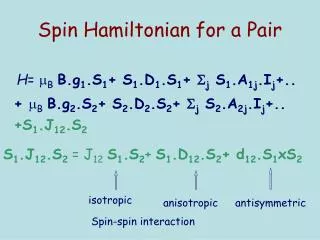
Spin Hamiltonian for a Pair. H = B B.g 1 .S 1 + S 1 .D 1 .S 1 + j S 1 .A 1j .I j +. + B B.g 2 .S 2 + S 2 .D 2 .S 2 + j S 2 .A 2j .I j +. +S 1 .J 12 .S 2. S 1 .J 12 .S 2 = J 12 S 1 .S 2 + S 1 .D 12 .S 2 + d 12 .S 1 xS 2. isotropic. anisotropic. antisymmetric.

E N D
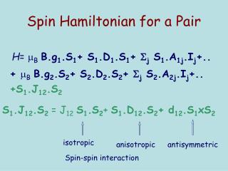
Spin Hamiltonian for a Pair H= BB.g1.S1+ S1.D1.S1+ j S1.A1j.Ij+.. + BB.g2.S2+ S2.D2.S2+ j S2.A2j.Ij+.. +S1.J12.S2 S1.J12.S2 = J12S1.S2+ S1.D12.S2+ d12.S1xS2 isotropic anisotropic antisymmetric Spin-spin interaction
SH Parameters for Pairs In the strong exchange limit, J>>D,d the total spin S=S1+S2 is a good quantum number: gS= c1g1+ c2g2 AS= c1A1+ c2A2 DS= d1D1+ d2D2+ d12D12 c1=(1+c)/2; c2= (1-c)/2; d1= (c++c-)/2; d2= (c+-c-)/2; d12= (1-c+)/2
Some numerical coefficients S1 S2 S c1 c2 d1 d2 d12 1/2 1/2 1 1/2 1/2 0 0 1/2 1 1 1 1/2 1/2 -1/2 -1/2 1 1 1 2 1/2 1/2 1/6 1/6 1/3 3/2 3/2 1 1/2 1/2 -6/5 -6/5 17/10 3/2 3/2 2 1/2 1/2 0 0 1/2 3/2 3/2 3 1/2 1/2 1/5 1/5 3/10
More coefficients S1 S2 S c1 c2 d1 d2 d12 2 2 1 1/2 1/2 -21/10 -21/10 13/5 2 2 2 1/2 1/2 -3/14 -3/14 5/7 2 2 3 1/2 1/2 1/10 1/10 2/5 2 2 4 1/2 1/2 3/14 3/14 2/7 5/2 5/2 1 1/2 1/2 -16/5 -16/5 37/10 5/2 5/2 2 1/2 1/2 -10/21 -10/21 41/42 5/2 5/2 3 1/2 1/2 -1/45 -1/45 47/90 5/2 5/2 4 1/2 1/2 1/7 1/7 5/14 5/2 5/2 5 1/2 1/2 2/9 2/9 5/18
And More S1 S2 S c1 c2 d1 d2 d12 1/2 1 1/2 -1/3 4/3 -- -- -- 1/2 1 3/2 1/3 2/3 0 1/3 1/3 1/2 3/2 1 -1/4 5/4 0 3/2 -1/4 1/2 3/2 2 1/4 3/4 0 1/2 1/4 1/2 2 3/2 -1/5 6/5 0 7/5 -1/5 1/2 2 5/2 1/5 4/5 0 3/5 1/5 1/2 5/2 2 -1/6 7/6 0 8/6 -1/6 1/2 5/2 3 1/6 5/6 0 4/6 1/6
Origin of the Spin-spin interaction • Through space (magnetic dipolar) • Through bonds (exchange)
Magnetic Dipolar J12dip= (B2/r3) [g1.g2- 3(g1.r)(g2.r)/r2]
Dipolar matrix in B2/r3 units gxxge 0 0 0 gyyge(1-3sin2) -3sin cos gyyge 0 -3sin cos gzzgegzzge(1-3cos2)
Decomposition of the interaction matrix J= (1/3)(Jxx+Jyy+Jzz) dxx=(Jyz-Jzy)/2 Dij=(Jij+Jji)/2
Dipolar interaction calculated r=2.5 Å r=3.5 Å r=4.5 Å J 18 7 3 D -3519 -1283 -603 E 28 11 5 dx -83 -30 -14 The values are given in 10-4 cm-1. gxx=gyy=2.2; gzz=2.0. The principal direction of D is parallel to the Mn-Cu direction
Origin of the Exchange Contributions J<g1g2Hexg1g2> D <n1g2Hexn1g2>2/2 D(g/g)2J d <n1g2Hexg1g2>/ d(g/g)J
A B Potential exchange- the case of non-degenerate terms 1. One half-filled orbital per ion: The effective Hamiltonian of the exchange interaction: one orbital per center: s-s molecule: Exchange integral (potentialenergy): 2.Non-degenerate terms: Many-electron exchange parameter (all bi-orbital interactions, half-filled orbitals): The effective Hamiltonian of the exchange interaction: many orbitals per center: Heisenberg-Dirac- Van Vleck model (HDVV model)
Ground Kinetic exchange-illustration for the simplest case of a dimer-one orbital/one electron per center P.W. Anderson, mechanism of the kinetic exchange: Charge transfer A*B, A*B AB Antiferromagnetic effect(J<0), singlet-triplet gap: |J |
-parameter of the isotropicexchange, incorporates contributions of all mechanisms: Lande’s rule for the intervals: Heisenberg-Dirac-Van Vleck (HDVV) model Full spin S numerates the energy levels (“good” quantum number): Further generalization: summation over all pairwise interactions ij in many-electron ions with full spinsSi and Sj Zeeman interaction (orbital part disappears in HDVV model): This result holds for any direction of the magnetic field H HDVV- isotropic model
Orbital configurations: degenerate ions Orbital configurations: non-degenerate ions Orbital doublets Orbital triplets Orbital triplets HDVV systems Non-Heisenberg systems When is the HDVV model applicable ?
HDVV modelisotropic interactions >>anisotropic interactions Heisenberg-Dirac-Van Vleck (HDVV) model The main condition of applicability-orbitally non-degenerate well isolated ground term in crystal field Under this condition the orbital angular momentum is strongly reduced andtheanisotropic terms arerelatively small (second and higher order corrections): Antisymmetric exchange: Local anisotropy: High order isotropic terms: biquadratic exchange, symmetric part of the anisotropic exchange tensor,etc
Il modello di Anderson A-C-B →A+-C-B- Lo scambio cinetico favorisce il singoletto Lo scambio potenziale il tripletto
Regole di Goodenough-Kanamori • Se gli orbitali magnetici si sovrappongono l’accoppiamento è antiferromagnetico • Se gli orbitali magnetici sono ortogonali ed hanno ragionevoli zone di sovrapposizione lo scambio è ferromagnetico • Se un orbitale magnetico sovrappone con un orbitale vuoto l’accoppiamento è ferromagnetico
Interazione di scambio Orbitali magnetici (quelli che hanno l’elettrone spaiato) con sovrapposizione diversa da zero: accoppiamento antiferromagnetico
Interazione di scambio (2) Orbitali magnetici ortogonali: interazione ferromagnetica (regola di Hund)
Interazione di superscambio (3) La frazione di elettrone trasferita nell’orbitale z2 polarizza gli spin degli altri elettroni spaiati, tenendoli paralleli a sé: accoppiamento ferromagnetico
Alcuni Esempi: Dimeri di Rame(II) > 96° < 96° R.D.Willett, D.Gatteschi,O.Kahn, Magneto-Structural Correlations in Exchange Coupled Systems, NATO ASI C140,Reidel, 1985
Rame(II)-Vanadile(IV) Indipendente dall’angolo J> 100 cm-1
Un po’ di MO - Hay-Thibeault-Hoffman + J’ è l’integrale di scambio, k sono integrali coulombiani
Il modello di Kahn J=j-ks2 J integrale di scambio s integrale di sovrapposizione
A test ground pair AF coupling J> 500 cm-1
Mixed Valence Manganese Dimers Manganese(III), d4, S=2 Manganese(IV), d3, S= 3/2 Antiferromagnetic coupling, S= 1/2
EPR Spectra of MnIII-MnIV The measurement of the g anisotropy possible at high frequency allows different fits of the hyperfine at low frequency 9 GHz 95 GHz 285 GHz
g Anisotropies in MnIII-MnIV giso gx gy gzDg bisimMe 1.9927 2.0022 1.9963 1.9796 0.0026 bispicenMe 1.9968 2.0055 1.9970 1.9878 0.0177 bisimH2 1.9920 2.0020 1.9935 1.9806 0.0214 bipy 1.9917 2.0005 1.9942 1.9850 0.0200 phen 1.9922 2.0002 1.9950 1.9814 0.0188 Un et al J Phys Chem B 1998, 102 10391
Coefficients for Clusters In the assumption of dominant isotropic exchange the coefficients for the spin hamiiltonian in an S multiplet can be obtained using recurrence formulae The coefficients depend on the intermediate spins
A trinuclear cluster c1(S1S2S12S3S)=c1(S12S3S)c1(S1S2S12) c2(S1S2S12S3S)=c1(S12S3S)c2(S1S2S12) c3(S1S2S12S3S)=c2(S12S3S) d1(S1S2S12S3S)=d1(S12S3S)d1(S1S2S12) d2(S1S2S12S3S)=d1(S12S3S)d2(S1S2S12) d3(S1S2S12S3S)=d1(S12S3S) d12(S1S2S12S3S)=d1(S12S3S)d12(S1S2S12) d13(S1S2S12S3S)=d12(S12S3S)c1(S1S2S12) d23(S1S2S12S3S)=d12(S12S3S)c2(S1S2S12)
Resonance fields for S states H(MM+1)=(ge/g)[H0+(2M+1)/D’/2]; D’=(3cos2-1)D/(geB)
HF-EPR Provides the Sign of D Negative D:±S lie lowest Easy axis type anisotropy At low T only the -S-S+1 transition is observed
An Example: Cu6 Ground S= 3 state
Single-Molecule Magnets • In molecular clusters with large spin S and Ising type anisotropy the magnetization relaxes slowly at low temperature • Intermediate behavior between classic and quantum magnets • HF-EPR is unique tool for determining the axial and transverse magnetic anisotropy
MS=-10 Easy axis of magnetization MS= 10 The first single molecule magnet: Mn12-acetate top view S4||z Prepared by a comproportionation reaction: T. Lis Acta Cryst.1980, B36, 2042. Mn(AcO)2•4H2O + KMnO4 in 60% v/v AcOH/H2O [Mn12O12(OAc)16(H2O)4]·2AcOH·4H2O lateral view z Manganese(IV) (s = 3/2, 3d3,) Manganese(III) (s =2, 3d4) Oxygen Carbon Ground state S = 8*2 - 4*3/2 = 10 Msaturation = 2.S = 20B
Very High Field EPR Spectra of Mn12acetate exp 525 GHz T= 30 K
Which are the conditions for tunneling? • The two wave functions must overlap • A transverse field must couple the two wavefunctions • The coupling splits the two states: tunnel splitting • The larger the tunnel splitting the higher the tunnelling probability
Zero Field EPR of Mn12Ac 9 8 10 9 8 7
Local Probes • Electron spin → EPR • Nuclear spin → NMR, NQR • Muon spin → μSR • Neutron spin → PND, INS Endogenous Exogenous