Download
1 / 46
510 likes | 872 Views
Reconstruction and Representation of 3D Objects with Radial Basis Functions. Carr et al. SIGGRAPH 2001 Presented by Yuntao Jia. Problem. Given a set of points Define an implicit function , such that: Surface is defined by the zero set of f. Constrains.

E N D
Reconstruction and Representation of 3D Objects with Radial Basis Functions Carr et al. SIGGRAPH 2001 Presented by Yuntao Jia
Problem • Given a set of points • Define an implicit function , such that: • Surface is defined by the zero set of f
Constrains • f(x) = 0 is a trivial solution • Add off-surface normal points to constrain the solution further
Off-Surface Normal Points • For each point, add two more points defining the inside and outside
Off-Surface Normal Points • Create points • New constrains
Choice of Parameters • is chosen as the distance of the new point from , signed distance function • must be chosen such that the displacement to the new point doesn’t intersect other parts of the surface
Generating Normals • Input is a point cloud, no normals • Generate normals as per [Hoppe 92] • Estimation from plane fitted to neighborhood • Additionally, use consistency and/or scanner positions to resolve ambiguities • If fails, don’t define off-surface normal points
Find the Implicit Function • Given a set of distinct nodes and a set of function values , find an interpolant s, such that
The interpolant is choose from , the Beppo-Levi space of distributions on with square integrable second derivatives • Square integrable means • is the space of functions in whose second derivatives fall off quickly
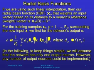
Radial Basis Functions • [Duchon 77] shown that the smoothest intepolant in is • It is a particular example of Radial Basis Functions:
Radial Basis Functions • p(x) is a low degree polynomial • are real coefficients • || is the Euclidean norm in • , the basis function, is a real function • Thin plate spline function • Guassian • Biharmonic and triharmonic splines
Radial Basis Functions • For biharmonic spline RBF, • B is symmetric and invertible under very mild conditions
Non-Compact Support • Biharmonic spline RBF • Pros • Suitable to non-uniformly sample data • Handle holes • Cons • A is not sparse, more computation and not scalable
Fast Methods • Approximated with Fast Multipole Method (FMM) • Cluster RBF centers into a hierarchy • Approximate evaluation for cluster far away • Direct evaluation for clusters near by • Reduce both storage and computation
RBF Center Reduction • Use fewer centers to achieve desired accuracy • A greedy algorithm • 1. Choose a subset of centers, fit a RBF • 2. Evaluate the residual, • 3. If < desired accuracy then stop • 4. Add new centers where is large • 5. Refit RBF and goto step 2
Noisy Data • Consider both interpolation and smoothness • measures the smoothness, is the weight • The linear system changes to
Noisy Data RBF approximation of a noisy LIDAR data
Surface Evaluation • A marching tetrahedra variant, optimized for surface following • Avoid RFS evaluation at a grid of voxels • Start from several seed points • Wavefronts of facets spread out across surfaces • Stop when intersect the bounding box
Surface Evaluation Iso-surfacing a RBF from a single seed point, wavefront marked by red.
Fast Multipole Methods (FMM) • Introduced by Rokhlin & Greengard in 1987 • One of the 10 most significant advances in computing of the 20th century • Speed up matrix-vector products of a particular type • Above sum requires O(MN) operations • For a given precision, it can be computed within O(M+N) using FMM
Fast Multipole Methods (FMM) • To solve a linear system • Requires O(N^3) using Gauss eliminations • Iterative method (e.g. conjugate gradient method) with FMM requires O(kNlog(N)) where k is the # of iterations and k<<N
Fast Multipole Methods (FMM) • Middleman • No space partitioning • Single Level Methods • Simple space partitioning • Multilevel FMM • Hierarchical space partitioning • Adaptive FMM • Data dependent space partitioning
Near Field and Far Field • S • Singular • Multipole • Outer • Far Field • R • Regular • Local • Inner • Near Field
Electronic Fields • The potential at X(x,y) due to a charge at x0
Fast Multipole Method • Initialization • create the spatial data structure (e.g. octree) and distribute points into cells
Upward Pass • For each finest/lowest level box, accumulate multipole expansions from points in it to its center • Expansion for boxes at higher levels are formed by merging expansion from their children boxes
Downward Pass 1 • At each level, for any box, we translate multipole expansions from its interaction boxes to itself as local expansions
Downward Pass 2 • Each box has local expansions contributed from its interaction lists • Start from highest level, we translate local expansions to the children level and add it to the children’s expansions
Final Summation • Every box has a local expansion including contributions from all boxes except its neighbors • First evaluation local expansion at target point • Add up contributions from source points in neighbors boxes using direct evaluation
Complexity • Create spatial data structure N • Create multipole expansions Np • p is the # of terms in the expansion • Multiple expansions to local expansions 29*N*p^2 • Evaluation of local expansion Np • Direct evaluation of neighbors 9Ns • s is the # of source points in a box
Reference • Reconstruction and Representation of 3D Objects with Radial Basis Functions. J. C. Carr, R. K. Beatson, J.B. Cherrie T. J. Mitchell, W. R. Fright, B. C. McCallum and T. R. Evans. ACM SIGGRAPH 2001, Los Angeles, CA, pp67-76, 12-17 August 2001. • Notes by Bolitho on [Carr et al 2001]. http://www.cs.jhu.edu/~misha/Fall05/ • Fast Multipole Methods (FAM04) Tutorial Lectures. Nail Gumerov and Ramani Duraiswami. http://www.cscamm.umd.edu/tutorials/index.htm • R. K. Beatson and L. Greengard. A short course on fast multipole methods. In M. Ainsworth, J. Levesley, W.A. Light, and M. Marletta, editors, Wavelets, Multilevel Methods and Elliptic PDEs, pages 1–37. Oxford University Press, 1997. • Many slides and pictures in this presentation are borrowed from those references. Q & A?