Download
1 / 10
100 likes | 108 Views
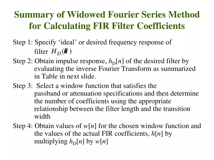
Summary of Widowed Fourier Series Method for Calculating FIR Filter Coefficients. Step 1: Specify ‘ideal’ or desired frequency response of filter

E N D
Summary of Widowed Fourier Series Method for Calculating FIR Filter Coefficients Step 1: Specify ‘ideal’ or desired frequency response of filter Step 2: Obtain impulse response, hD[n] of the desired filter by evaluating the inverse Fourier Transform as summarized in Table in next slide. Step 3: Select a window function that satisfies the passband or attenuation specifications and then determine the number of coefficients using the appropriate relationship between the filter length and the transition width Step 4: Obtain values of w[n] for the chosen window function and the values of the actual FIR coefficients, h[n] by multiplying hD[n] by w[n]
Summary of ideal impulse response of standard frequency selective filters
Summary of Important Features of Common Window Functions Window Representation Expression Rectangular wR[n] 1 Hanning whn [n] 0.50 + 0.50 cos{2n/(N)} Hamming whm [n] 0.54 + 0.46 cos{2n/(N)} Blackman wb [n] 0.42 +0.50 cos{2n/(N-1)} +0.08 cos{4n/(N-1)} Order of filter = N = where c the coefficients depend on type of windows being used as in table next slide
Summary of Important Features of Common Window Functions….Cont Window Transition Passband Stopband Width Ripple Attenuation (dB) (normalized) (dB) (maximum allowed) Rectangular 0.9/N 0.7416 21 Hanning 3.1/N 0.0546 44 Hamming 3.3/N 0.0194 53 Blackman 5.5/N 0.0017 75
Example:Design a low-pass FIR filter to meet the following specs:Pass band edge frequency: 1500 HzTransition width: 500 Hz.Stop-band attenuation AWS= > 50 dBSampling frequency fs = 8000 Hz. • Problem Statement: • Meaning of given specifications are: • Sampling frequency fs = 8000 Hz. • Pass band edge frequency: fc =1500/8000 • Transition width f = 500/8000. • Stop-band attenuation AWS= > 50 dB
Design considerations contd… • The filter function is • Because of stop-band attenuation characteristics, either of the Hamming, • Blackman or, • Kaiser windows • can be used. • We use Hamming window: • whm[n] =0.54 + 0.46 cos{2n/(N-1)}
Design considerations contd… • f = transition band width/sampling frequency = 0.5/8 =0.0625 = 3.3/N. • Thus N = 52.8 53 i.e. for symmetrical window • –26 n 26. • fc’ = fc + f/2 = (1500+ 250)/8000 = 0.21875. • Calculate values of hD [n] and whm[n] for • –26 n 26 • Add 26 to each index so that the indices range from 0 to 52. • Plot the response of the design and verify the specifications.
Calculations: • c = 2fc’= 1.3745 • 2 fc’=1.3745/ = 0.4375 • hD(n) = fc’[sin(nc)/ nc] • wn = [0.54 + 0.46cos(2n/N) • The input signal to the filter function is a series of pulses of known width but of different heights manipulated as per the window function. • The overall is the multiplication of two.
Calculations… h(n) = hD [n] w D[n] = 0.4375 {[sin(nc)/ nc]} x {[0.54 + 0.46cos(2n/N)} at n=0, since sin(nc)/nc = 1, and cos(0) = 1; h(0) = 0.4375 x[0.54 + 0.46] = 0.4375. Again since 2 fc’ / c = 1/ h(n)= [sin(1.3745n)/n] [0.54 +0.46cos(2n/53)]