Download
1 / 42
420 likes | 524 Views
Solar Thermal Systems Cameron Johnstone Department of Mechanical Engineering Room M6:12 cameron@esru.strath.ac.uk. 60 million AGR’s. 30%. Not quite. Hydro. Wind & Wave. Bio-fuels. Do All Energy Resources Originate from the Sun ?. 47%. 23%. 0.21%. 0.06%. 7x 10 -9 %.

E N D
Solar Thermal Systems Cameron Johnstone Department of Mechanical Engineering Room M6:12 cameron@esru.strath.ac.uk
60 million AGR’s 30% Not quite Hydro Wind & Wave Bio-fuels Do All Energy Resources Originate from the Sun ? 47% 23% 0.21% 0.06% 7x 10⁻⁹% 12.7 MW / 4kg/s Oil
Solar Data • Statistics: diameter of Sun 1.39 x 10⁶ km diameter of Earth 12.7 x 10³ km distance from Earth 1.5 x 10⁸ km transmission time 500s • Nuclear fusion at Sun => Surface Temp. 5800K Core Temp. 8 x 10⁶ - 40 x 106 K Density = 80 / 100 x water
The Sun • The ultimate source of energy in the sun is a nuclear fusion reaction, heating core to about 107 K • Energy from fusion reaction emitted as X-rays, gamma rays and high-energy particles known as neutrinos • Radiation heats passive layers of gas in sun’s outer atmosphere to around 5800K. These layers then radiate energy to the earth.
Solar Data • Rotation Earth = 1/ 24 hours Sun = 1/ 4 weeks 27 days @ equator 30 days @ polar regions • Radiant Flux Density (RFD) (Irradiance or Insolation) 1.35kW/m2 (outer space) 1 kW/m2 (sea level) - due to Albedo effect and absorption in atmosphere
Solar Spectral Emission Wavelength band => 0.3 m - 2.5 m (shortwave) Makeup: < 0.4m (ultraviolet) 9% of RFD 0.4 m < < 0.7 m (visible) 45% of RFD > 0.7 m (infrared) 46% of RFD
Black Body Radiation • Radiant energy reaching the earth from the sun closely approximates radiation from a black body at a temperature of about 5800 K. • A back body is an object that radiates energy according to the following equation: (Stefan-Boltzmann constant = 5.67× 10⁻⁸W/m2K4) • Representing the maximum possible energy emitted by a body at temperature T. • In reality the quantity of energy emitted by all real bodies will be less than this.
Photons • The radiant energy from the sun can be thought of as discrete “packets” of energy known as a photons • The energy carried by an individual photon (E) is given as the product of its frequency v and a quantity known as Planck’s constant (h = 6.626 × 10⁻³⁴ Js) • This equation shows that photons and consequently radiation with a high frequency has the greatest energy.
Photons • Wavelength and frequency are related by the equation: • Substituting for for frequency: • The shorter the wavelength (higher frequency) the greater the energy of the radiation/photon.
Planck’s Law • Wavelength or frequency of emitted radiation is related to the temperature of the emitting body by Planck’s law, this gives the rate of energy (Q) radiated at any wavelength, λ(μm), by a black body of temperature T (K). • The quantity Qλ is known as the emissive power of the black body. C1- 3.742 x 10⁸ W m4/m2 C2- 1.44 x 10⁴ K
Establishing the Sun’s equivalent ‘Black Body’ Temperature • Wien’s Displacement Law m = Cw Tabs where: m = Wavelength of max. energy (m) Cw = Wien’s constant 2820 (m K) T = Absolute temp. (K) For global irradiance m ≈ 0.5 m
Atmosphere X2 Earth X1 x2 > x1 Solar energy: Air mass Air mass (AM) = 1/ Cos Air mass 1 at Equator Air mass 1.5 at latitudes 48.5 Air mass 2 at latitudes 60
Components of Irradiance For perpendicular surfaces Beam (Gb) => 0% - 90% Diffuse (Gd) => 10% - 100% Total irradiance G = Gb + Gd For inclined surface Gb = Gb x Cos Total irradiance G = Gb + Gd
Angles associated with the Solar Plane Zenithangle = angle of decline from the overhead position. Azimuth angle = angle of difference from solar noon. Characteristics of Solar Materials All materials have the following characteristics Transmission () Absorptance () Reflectance () For any material: + + = 1
3 1 Solar Collector Solar power absorbed into collector Useful power from collector 2 Power loss from collector Solar collector components Protective cover (c) - high value Absorber/collector plate (p)- high value Shading device (optional) - high value
Absorbed power in a solar collector Given by (1): QP = G A cp where: QP = absorbed power (W) G = total irradiance (W/m2) A = area of solar collector (m2) c = transmission factor of cover p = absorptance factor of collector plate
Power loss in a solar collector Given by (2): QL = U A (Tc - Ta) where: QL = power lost (W) U = collector U value (W/m2K) Tc = temperature of collector plate (K) Ta = temperature of ambient (K)
Solar Collector 3 1 Solar power absorbed into collector Useful power from collector 2 Power loss from collector Power supplied by a solar collector Derived from Hottel - Whillier equation (3): = (1) – (2) QS = GA cp - [UA (Tc - Ta)]
Solar collector performance characterisation The stagnation temperature method Qsup = 0 loss from collector is equal to the power absorbed at the collector plate: Qabs = Qloss For a conventional flat plate collector, the collector temperature (Tc) at stagnation: GA cp= UA (Tc- Ta) Tc= GA cp+ Ta UA
Gb Concentrator Collector Solar concentrators Focusing beam irradiance (Gb) incidental on a large surface area onto a smaller absorbing area. Effective operation requires: - complex tracking and control systems
Concentration ratio of concentrator • Concentration Ratio (X) X = Aa Ac • Where: Aa - projected area of concentrator (2 dimensional image) Ac - collector area
Gb Concentrator Collector Power supplied to an evacuated collector (1) Power Absorbed (Qabs) Qabs = Gb Aaa g c Where: Gb - beam irradiance (W/m2) a - reflectivity of parabolic surface g- transmissivity of glazed cover c - absorbtivity of collector
Solar Collector 3 1 Solar power absorbed into collector Useful power from collector 2 Power loss from collector Power loss from an evacuated collector (2) Qloss = Ac [ Tc4 - Tg4 ] Where: - emissivity of collector surface - Boltzman’s constant (5.669 x 10⁻⁸ W/m2K4) Tc - collector surface temperature (K) Tg - glazing temperature (K)
Power supplied by the evacuated collector (1) – (2) Power supplied (Qsup): = Qabs – Qloss = ( Gb Aaagc ) – ( Ac [ Tc4 - Tg4 ] ) Performance appraisal/ comparison under stagnated conditions: Qsup = 0 Qabs = Qloss Gb Aaagc = Ac [ Tc4 - Tg4 ] Stagnation temperature is: Tc4 = Gb Aaagc + Tg4 Ac
Unglazed collector Single glazed collector Efficiency (%) Double glazed collector Evacuated concentrator collector Temperature rise T (°C) Collector efficiency Defined as power delivered (useful power) divided by Gtot
Solar water heating example • Analysis is an iterative process because so many variables including: • solar radiation intensity, • temperature of the solar collector, • effectiveness and efficiency of the heat exchange processes • temperature of the hot water in the tank. • Calculate the resulting heat transfer rate and energy balance at each time step • Hottel-Whillier and Bliss equation has (F) component
UAT Twater mCpT Eff. GA Solar water heating example • A 3m2 flat plate solar collector with the following characteristics is used to heat a 72 litre hot water tank. If there is no draw off of water calculate: • i) the maximum stagnation temperature reached, • ii) the maximum water temperature within the storage tank, and • the mean hourly collector efficiency • collector “U” value (W/m2 K) 3.5 • collector absorptance () 0.9 • transmissivity of cover () 0.74 • effectiveness of collector plate (F) 0.9 • initial water temperature (C)10 • density of water (kg/m3) 1000 • specific heat capacity of water (J/kg K) 4200 • water flow rate (l/s) 0.02
Solar Skins/ Walls Solar skins/ walls should be a net contributor of energy to a building. Can be of two types: Thermal Mass or Phase Change storage Thermal mass storage: Sensible heating, therefore for solar energy input – collector temperature increase results in system losses increasing. Materials: Rock/ concrete 1 < Cp < 1.4 kJ/ kgK Water Cp = 4.2 kJ/kgK
Solar Skins/ Walls Phase Change Storage: Sensible and Latent heating • At PC temperature: While energy input is maintained - Temperature remains constant - Losses remain constant, improving system efficiency. Materials: CaCl2 saturated solution changes phase (solid to liquid) at 28C Latent heat 198 MJ/ m3 Durability: Proven to over 6000 complete PC cycles ?
Solar Skins/ Walls: Performance appraisal Since heating demand does not occur at time of solar availability, time lags are introduced by using thermal capacity.
Solar Skins/ Walls: Time lag Associated time lags as demonstrated on Strathclyde’s Solar Residences
Solar Skins/ Walls: Performance Appraisal Temperature swing is cyclic between a maximum (solar noon) and minimum (early morning) every 24 hour period. For solar applications the frequency of temperature swing (n) is a 24 hour period, and determined as follows: n = 1/ time (sec) For solar wall applications n = 1.157 x 10⁻⁵
Solar Skins/ Walls: Performance Appraisal Flux absorbed at surface penetrates into the wall and gets diffused. Diffusion rate of is referred to as the Thermal Diffusivity () and calculated as follows: = k /Cp where: = Thermal diffusivity (m2/s) k = Thermal conductivity of wall (W/mK) = Density of wall material (kg/m3) Cp = Specific heat capacity of wall (J/kg K)
Solar Skins/ Walls Performance Appraisal The velocity at which energy will travel through the wall is determined by the thermo-physical properties of its construction. Important when designing the thickness of the wall so peak thermal flux occurs at the time of peak heating demand. The velocity (v) of the thermal wave is given by: v = 2 (n)1/2
Solar Skins/ Walls Performance Appraisal The temperature at a point through the wall fluctuates around the mean external wall surface temperature experienced over the 24 hour period, Tmean at the external surface is: Tmean = 1/2 (Tmax + Tmin) The specific temperature fluctuation (T) above or below Tmean at a distance (x) metres into the wall is: T = T e [ -x (n / )1/2 ] where: T - amplitude of the wall surface temperature from Tmean over the 24 hour period i.e. Tmax - Tmean(C) x - distance from external surface of wall (m) n - frequency of temperature swing - thermal diffusivity (m2/s)
Solar Skins/ Walls Performance Appraisal Maximum and minimum temperatures at a specific point within the wall (Tx) is calculated by adding or subtracting the temperature swing to/from the mean surface temperature : Tx = TmeanT The Energy (E) stored within the wall is: E = m Cp (Tmean – Tamb) Where: E = energy (j) m = mass of wall (kg) [volume x density] Cp = Specific heat capacity of wall material (j/kgC) Tamb = average outside air temperature over the day
Solar Skins/ Walls: Performance appraisal Solar walls assessed via net energy contributions: Heat flux transferred relative to solar flux available.
Solar Skins/ Walls: Performance appraisal Flux capture derived via the Hottel-Whillier Eqn. to give negative values in sufficient irradiance (energy contribution) and positive values in no or low irradiance (energy loss). Qres = Uc (Tabs - Ta)- Gv where: Qres = Resultant power flux (W/m2) Gv = Incidental irradiance (W/m2) Uc = Collector “U” value (W/m2K) Tabs = Collector absorber temperature Ta = Outside air temperature
Solar Skins/ Walls: Performance appraisal This can be rewritten as: Qres / (Tabs-Ta) = Uc - ( Gv / (Tabs - Ta)) Since Uc and remain constant, plotting Qres / (Tabs-Ta) against Gv / (Tabs - Ta) over an extended period of time and under a variance of irradiance conditions gives: Y = mX + C Analysis of this distribution can determine the following characteristics: m = collector efficiency () C = ‘Udark’ value (‘U’ value in no irradiance)
‘Udark’ ‘Ueffective’ m = eff. Solar Skins/ Walls: Performance appraisal ‘U’ values ‘Udark’ Wall performance without solar exposure. ‘Ueffective’ Wall performance when exposed to the sun
Solar Skins/ Walls: Performance appraisal The summation of all the plotted Qres / (Tabs-Ta) divided by the number of values plotted (n) gives an average U value (Ueff) for the wall examined under a variety of conditions. Ueff is defined as follows: Ueff = Qres / (Tabs-Ta) n “Good”, solar walls have negative ‘Ueff’ values indicating they contribute more power than is lost from them over the evaluation period.