Download
1 / 16
160 likes | 225 Views
Cluster Analysis of AMSR-E Brightness Temperatures. Danny Braswell and Roy Spencer 23 September 2014. Defining cluster analysis.

E N D
Cluster Analysis of AMSR-E Brightness Temperatures Danny Braswell and Roy Spencer 23 September 2014
Defining cluster analysis • In a general sense, cluster analysis is the grouping of a set of items into subsets of items with similar characteristics. For example, in a restaurant you could group (cluster) patrons based what they ordered, or whether or not they added salt to their food, or even the color of their clothes. Another way would be to cluster them based on separation distance, e.g. those sitting together at each table. • Separation distance is one of the more common ways of clustering items. This can be in a 2 or 3 dimensional real space or in a higher order multi-dimensional space. • Accounting for the distance is usually done in one of two ways: absolute distance or squared distance. • Squared distance places progressively greater weights on larger separations, and is the more commonly used.
Defining cluster analysis (cont) • For our purposes, we use “cluster analysis” to mean the dividing of M points in N dimensions into K clusters so that the within-cluster sum of squares is minimized. • Each cluster is defined by the coordinates of its centroid. • As a simple example in 2-D, consider random points on a square grid. • Each point is defined by its (x,y) coordinates.
Random points on a square grid 10,000 points
Random points on a square grid classified into 4 clusters Cluster centroids marked in red
Random points on a square grid classified into 6 clusters Cluster centroids marked in red
Clustering of AMSR-E Tbs • For AMSR-E, a point is defined by 9 simultaneous AMSU channel differences computed from the 10 channels: - 10V, 10H - 18V, 18H - 23V, 23H - 36V, 36H - 89V, 89H • Reference channel for differences: 18V • 9 dimensions - each channel difference is considered a dimension • Differences used to remove temperature signal • 10 clusters • Used K-means algorithm by Hartigan and Wong (ref at end) to perform clustering
AMSR-E Data Used • AMSR-E Level 2A (v12) • Land only • ASC/DSC orbits combined • Days: 1/15/2008, 6/15/2008
Average Tbs for each cluster 1 6 4 2 7 Tb (K) 9 8 5 3 10 Channel
Clusters 1, 2 2 - snow 1 - dense veg
Clusters 3, 4 4 – snow/storms 3 – glacial ice
Clusters 5, 6 6 – sparse veg 5 – deep snow
Clusters 7, 8 8 - snow 7- marginal desert/sea ice
Clusters 9, 10 10 – glacial ice 9 – desert/glacial ice
Reference for:K-means Clustering Algorithm • Hartigan, J. A.; Wong, M. A. (1979). "Algorithm AS 136: A K-Means Clustering Algorithm". Journal of the Royal Statistical Society, Series C28 (1): 100–108. • Fortran 77 subroutine asa_136.favailable from: http://lib.stat.cmu.edu/apstat/136