Download
1 / 30
300 likes | 418 Views
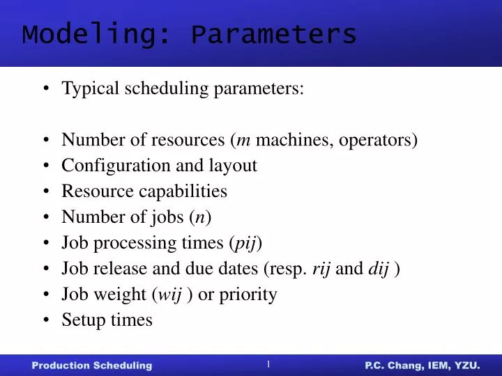
Modeling: Parameters. Typical scheduling parameters: Number of resources ( m machines, operators) Configuration and layout Resource capabilities Number of jobs ( n ) Job processing times ( pij ) Job release and due dates (resp. rij and dij ) Job weight ( wij ) or priority

E N D
Modeling: Parameters • Typical scheduling parameters: • Number of resources (m machines, operators) • Configuration and layout • Resource capabilities • Number of jobs (n) • Job processing times (pij) • Job release and due dates (resp. rij and dij ) • Job weight (wij ) or priority • Setup times
Modeling: Objective function • Objectives and performance measures: • Throughput, makespan (Cmax, weighted sum) • Due date related objectives (Lmax, Tmax, ΣwjTj) • Work-in-process (WIP), lead time (response time), finished inventory • Total setup time • Penalties due to lateness (ΣwjLj) • Idle time • Yield • Multiple objectives may be used with weights
Modeling: Constraints • Precedence constraints (linear vs. network) • Routing constraints • Material handling constraints • (Sequence dependent) Setup times • Transport times • Preemption • Machine eligibility • Tooling/resource constraints • Personnel (capability) scheduling constraints • Storage/waiting constraints • Resource capacity constraints
Machine configurations: • Single-machine vs. parallel-machine • Flow shop vs. job shop Processing characteristics: • Sequence dependent setup times and costs • length of setup depends on jobs • sijk: setup time for processing job j after k on machine i • costs: waste of material, labor • Preemptions • interrupt the processing of one job to process another with a higher priority
Generic notation of scheduling problem • Machine Job Objective • characteristics characteristics function • for example: • Pm | rj, prmp | ΣwjCj (parallel machines) • 1 | sjk | Cmax (sequence dependent • setup / traveling salesman) • Q2 | prec | ΣwjTj (2 machines w. different speed, precedence rel., weighted tardiness)
Scheduling models • Deterministic models • input matches realization • vs. • Stochastic models • distributions of processing times, release and due dates, etc. known in advance • outcome/realization of distribution known at completion
Static V.S. Dynamic • Static Assume all the jobs are ready at the beginning which means ai=0 • Dynamic Each job with a different arrival time. Which ai≠0
Large Scale Problem (man-made) approach Upper Bound (Heuristic) available solution space Optimum unavailable solution space Lower Bound (Release Constraints) approach
Performance Measure • Completion Time • Cmax = Max Ci = C6 • 指工件集合s中,最晚之完工時間,即指Cmax. (Makespan) • Minimize Inventory • fi : 庫存降低 • fi = Ci – ai ( Static Problem : ai=0) • Satisfy Due Date • Tardiness = Max(Ci-di , 0 ) • Earliness = Max(di-Ci , 0 ) • JIT = Ci-di • Bi-criteria Multi-Objective (flow time = waiting time + process time)
1 2 3 4 0 5 8 12 13 Compute flow time 5 3 4 1 5 5 5 5 3 3 3 4 4 1 第i順位之Pi
Gantt Chart 3 2 1 5 4 6 jobs are ready d3 c3d1c2 d2 c1d4c5c4d5 d6 = c6 flow time tardiness c2 – a2 c4 > d4
Scheduling Problem Representation 4 / 1 / (n / m / o ) objective function # machine # job . . . . .
Example: A factory has receive 4 different orders as follows • Please assign the production sequence of the 4 jobs to satisfy: • Due Date • Min Inventory
Sol. 1. Using FCFS (First come first serve) 1-2-3-4 1 2 3 4 0 5 8 12 13
Sol. • Using EDD (Earliest Due Date) 4-2-3-1 4 2 3 1 0 1 4 8 13
Sol. • Using SPT (Shortest Processing Time) The same with EDD Optimum 4-2-3-1 4 2 3 1 0 1 4 8 13 • EDD – Due Date – Tmax • SPT – Inventory - Flow time
Bi-criterion SPT Frontier EDD
HW. 5 / 1 / Draw the Frontier when
Dynamic Problem Example: 4 / 1 /
Sol. Ck > ai , C1≧ a2 - no idle time Else, if ai > Ck, a2 > C1 - idle 1. Using Job index 1-2-3-4 1 2 3 4 0 3 8 11 15 16 3-5 3-2 3-4 • 5-2 5+1 5-1 =18 • 3 3 3 = 9 • 4 4 = 8 • 1 = 1 • 36 or
Sol. 2. Using SPT. EDD 4-2-3-1 4 2 3 1 0 4 5 8 12 17
Sol. 3. Using FCFS then SPT (ESPT) 從Available jobs找SPT 3-4-2-1 3 4 2 1 0 2 6 7 10 15 Static (SPT) 排了工件3之後,Dynamic問題變為Static,所以SPT 每個工件輪流排第一來比較
Ex:ESPT • find Min • for min
Sol. 1. Using Job index 1-2-3-4 1 2 3 4 0 3 8 11 15 16
Sol. • Using SPT • Using EEDD (next slide) 4-2-3-1 4 2 3 1 0 4 5 8 12 17
Ex:EEDD • find Min • for min let • Return 3
HW. 1. 5 / 1 / 2. 5 / 1 / Find an optimal solution!