Download

1 / 26
260 likes | 502 Views
Contents Introduction Matrix Multiplication Partitioned Matrices Powers of a Matrix Transpose of a Matrix Theorems and Proofs Application of Matrix Multiplication Questions Links. The Matrix… What is a matrix?

E N D
Contents • Introduction • Matrix Multiplication • Partitioned Matrices • Powers of a Matrix • Transpose of a Matrix • Theorems and Proofs • Application of Matrix Multiplication • Questions • Links
The Matrix… What is a matrix? A matrix is a rectangular array of numeric or algebraic quantities subject to mathematical operations, or a grid of numbers. Row → 2 4 7 1 -3 6 ↑ Column The size of this matrix is m × n, where m represents the number of rows and n represents the number of columns. For example, the matrix shown above is a 2×3 matrix.
Matrix Multiplication Scalar Multiplication Consider the following If s is a scalar and A is a matrix 1 5 s = 2, and A = 4 3 2 1 1 5 2(1) 2(5) 2 10 sA = 2 * 4 3 = 2(4) 2(3) = 8 6 2 1 2(2) 2(1) 4 2 Rule: if s is a scalar and A is a matrix, then the scalar multiple sA is the matrix whose columns are s times the corresponding entries in A. In other words, you take the scalar and multiply it with every number in the matrix. Theorem: If r and s are scalars, then (r + s)A = rA + sA andr(sA) = (rs)A.
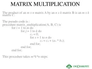
Matrix MultiplicationBefore you multiply a matrix by another matrix, you need to check the compatibility of the two matrices. The number of columns (n) in A must equal the number of rows (m) in B in order to carry out the matrix multiplication.Example 1A = 2 5 B = 3 1 7 1 3 8 2 4 m × n m × n 2×2 2×3You can see that the number of columns of A matches the number of rows of B. (Later on, you will see that the size of matrix AB will be m of A × n of B). Example 2A = 2 5 B = 3 1 7 1 3 8 2 44 1 2 2×2 3×3 Obviously, n of A ≠ m of B and thus they are not compatible for multiplication.
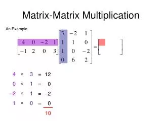
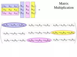
Example 3 Find the product AB from the following matrices A = 1 0 -2 5 3 -1 B = 6 3 4-3 -7 2 A is a 2×3 matrix and B is a 3×2 matrix, and they are compatible. To get the final product, we will be sequentially multiplying each row in one matrix by the corresponding column in another matrix. In this example, we take the first row of A and first column of B, multiply the first entries together, second entries together, and third entries together, and then add the three products. 1 0 -2 * 6 = 1(6) + 0(4) + (-2)(-7) = 20 4 -7
Example 3 cont. This sum is one of the entries in the product matrix AB; in fact, being the product of row 1 of A and column 1 of B, it is the (1,1)-entry in AB. Column 1 ↓ Row 1 → 20 # # # Then we continue in like manner; we multiply row 1 of A by column 2 of B. 1 0 -2 * 3 = 1(3) + 0(-3) + (-2)(2) = -1 -3 2 And its position in matrix AB is Column 2 ↓ 20 -1 ← Row 1 # #
Example 3 cont. Multiplying row 2 of A by column 1 of B gives 5 3 1 * 6 = 5(6)+3(4)+(1)(-7) = 35 4 -7 And its position in matrix AB is at row 2 and column 1. You can do the last multiplication of row 2 of A by column 2 of B by yourself. So the final answer is AB = 1 0 -2 * 6 3 = 20 -1 5 3 1 4 -3 35 8 -7 2 Handy trick: As we mentioned before, the size of matrix AB is 2×2 (A is a 2×3 matrix and B is a 3×2 matrix). AB ≠ BA (Can you see why?)
Partitioned Matrices Matrices can be written as partitioned matrices. Example 3 0 -1 -2 9 5 A = -6 -4 0 3 1 7 2 -5 4 8 0 1 Can also be written as a 2×3 partitioned matrix A =A11A12A13 A21A22A23 A11 = 3 0 -1 A12 = -2 9 A13 = 5 -6 -4 0 3 1 7 A21 = 2 -5 4 A22 = 8 0 A23 = 1
Multiplication of Partitioned Matrices Example 4 -6 5 1 -4 2 -2 1 -2 A = 3 2 1 4 0B = 3 7 0 -3 7 1 1 2 5 -1 3 A = A11A12B =B1 A21A22B2 AB = A11A12 * B1 = A11B1+ A12B2 = 15 -56 A21A22B2 A21B1+ A22B2 25 5 19 63
Powers of a Matrix If A is a n×n matrix and if K is a positive integer, then K can be raised to the power of A, as in AK and means that you can have K copies of A. Example A3 = A*A*A If we have A being nonzero, and X is in the set of real numbers, then AKX is like multiplying X by A repeatedly K times. However, if K = 0, then A0X should be X itself as A would be interpreted as the identity matrix. In this way, matrix powers end up being very useful in both theoretical and applied means. Transpose of a Matrix If we have a given matrix, A that is if the size mxn, then the transpose of it would be an nxm matrix and is denoted by AT. In other words, you take an initial row in the original matrix and make it a column in the transposed matrix, and vice versa with the rows. Let’s look at an example, A = , and if we follow the rules then AT =
Theorems and Proofs All right people, I know this is the part where it gets really technical, but in the true sense of achievement and comprehension of the concepts here, we believe this too is necessary. Theorem 1 Let A, B and C be matrices of the same size, and let p and q be scalars. a. A+B = B+A b. (A+B) + C = A + (B + C) c. A + 0 = A d. p(A + B) = pA + pB e. (p+q)A = pA + qA f. p(q A) = (pq) A The proof of all these equalities lies in showing that each of the matrices of the left hand side are equal in size to the matrix on the right hand side, and also by showing that entries in corresponding columns are equal. We already assumed that the matrices are of equal size at the start, so that is taken care of. As for the other condition, that seems to be satisfied with if we follow the analogous properties of vectors. For those of you who are not aware of these, here’s an example.
If the jth column of A, B, and C are aj, bj, and cj, respectively, then the jth columns of (A+B)+C and A+(B+C) are (aj + bj) + cj and aj + (bj + cj) respectively. Since the two vector sums are equal for each j, property (b) is verified. Moreover, because of the associative property of addition, we can say that A+B+C = (A+B)+C or A+ (B+C), and the same can be applied to the sum of four or more matrices. Theorem 2 If A is an p x q matrix, and of B and C have sizes for which the indicated sums and products are defined, then using some basic laws of arithmetic and some others we can also verify the following statements: a. A (BC) = (AB) C (associative law of multiplication) b. A (B + C) = AB + AC (left distributive law) c. (B+C)A = BA+ CA (right distributive law) d. r(AB) = (rA) B = A(rB) for any scalar r e. ImA = A = AIn (identity for matrix multiplication)
Proof Statements a to d are self explanatory and the basic laws of arithmetic stated are what verify them as well. As for statement e, the identity matrix is just and that multiplied by any matrix is the matrix itself. Example =(You should be able to see why that is correct) Theorem 3 Let A and B denote matrices whose sizes are compatible enough for the following sums and products. a. (AT )T = A b. ( A+B)T = AT + BT c. For any scalar p, (p A)T = p AT d. ( AB )T = BT AT
Proof Proofs of A to C are straight forward and thus omitted. For d, let’s look at this example. Let A = , B = , then (AB) = and (AB)T = Whereas, BT = and AT = . Moreover, BT AT = . Thus, as both the answers to the left hand side and the right hand side of the equation are the same, then the statement is proved.
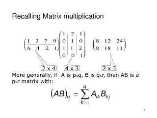
Theorem 4 Column - row expansion of AB If A is an mxn matrix and B is an nxp, then, AB = [col1 (A) col2 (A) … coln(A)] = col1(A) row1(B) + … + coln (A)rown(B) Proof For each row index i and column index j, the (i, j)- entry in colk (A) rowk (B) is the product of aik from colk(A) and bkj from rowk (B). Hence the (i,j)-entry in the sum shown in (1) is ai1 b1j + ai2 b2j + … + ain bnj (k=1) (k=2) (k=n) This sum is also the (i, j)-entry in AB, by the row-column rule.
Row - Column rule for Computing AB: If the product AB is defined, then the entry in row i and column j of AB is the sum of the products of corresponding entries from row i of A and column j of B. If (AB)ij denotes the (i, j)-entry in AB, and if A is an m x n matrix, then (AB)ij = ai1 b1j + ai2 b2j + … + ainbnj Warnings: Finally, there are a few things that we would like you to keep in mind. 1. In general, AB does not equal BA. 2. The cancellation laws do not hold for matrix multiplication. That is, if AB = AC. The it is not true in general that B = C. 3. If a product AB is the zero matrix, you cannot conclude in general that either A = 0 or B = 0.
Application of Matrix Multiplication Now, We are sure you must all be aware that matrix multiplication is not just a random concept that we learn in mathematics. It has many useful applications in everyday life and also in other branches of math. So now, we will spend some time looking over and trying to understand what exactly it is and where it is that matrix multiplication is applicable. The Matrix Application Ax = b As stated before, one of the most useful applications of matrix multiplication in math is in the matrix equation. The fundamental idea behind this equation is that in Linear Algebra we can view a linear combination of vectors as the product of a matrix and vector (a quantity specified by a magnitude and a direction). And it is in this fundamental concept that lies the existence of matrix multiplication. This is because a vector can be written in matrix notation and then multiplied to the other matrix to obtain one side of the equation and then carry out the appropriate operations and functions from there on end.
A formal definition stating this relationship is given below. Definition If A is a m x n matrix, with columns a(1),…,a(n), and if x is in the collection of all the lists of real numbers, then the product of Ax, is the linear combination of the columns of A using the corresponding entries in x as weights; that is, x1 Ax = [ a1 a2 … a(n)] * x2 = x1a1 + x2a2 + … + x(n)a(n) x(n) Note that Ax is defined only if the number of columns of A equals the number of entries in x.
Example For a given set of vectors, v1,v2,and v3 in the real set of number R, and the weights 3, -5, and 7, write up a linear combination by combining a matrix and a vector. Step 1 Write out the vector in matrix notation, v1, v2, v3 = [ v1 v2 v3] Step 2 Write out the weights as a column matrix as well, 3 3, -5 and 7 in a column matrix would equal -5 7 Step 3 Write them out side by side and multiply, 3 [v1 v2 v3] -5 = 3v1 – 5v2 +7v3 7 We can only multiply two matrices together when the columns of the first matrix equal the rows of the second.
Matrix Multiplication in Economics We gave you an example of how matrix multiplication could be used in math itself, but how about in real life, what benefit can it provide to us? Well, one of the major benefits is seen when scalar multiples and linear combinations can arise when a quantity such as 'cost; is broken down into several categories. The basic principle for the example concerns the cost of producing several units of an item when the cost per unit is known. {Number of units} * {Cost per unit} = {Total cost} Example A company manufactures two products. For $ 1.00 worth of product A, the company spends $ .40 on labor, $.20 on labor, and $.10 on overhead. For $1.00 worth of product B, the company spends $.30 on materials, $.25 on labor, and $.35 on overhead. Suppose the company wishes to manufacture x1 dollars worth of product A and B. Give a vector that describes the various costs the company will have to endure?
Step 1 .40 .30 A = .20 and B = .25 .10 .35 Step 2 The cost of manufacturing x1 dollars worth of A are given by x1*A and the costs of manufacturing x2 dollars worth of B are given by x2.B. Hence the total costs for both products are simply given by their products once again, .40 .30 [ x1 ] .20 + [ x2 ] .25 = x1*A + x2*B. .10 .35
Test 2 • 5. 2 -3 -4 1 -3 • -4 1 1 -1 0 • -4 -3 • 6. -1 3 4 0 -3 • 4 -2 3 -4 1 • 2 -3 2 -3 -1 • 7. -1 2 4 4 3 • -3 -3 4 2 -3 • -1 -1 1 1 -1 • 8. -1 2 3 4 • -1 2 2 -4 • -2 0 Questions Here are some matrix multiplication problems you can practice with. And of course, you can check your answers in the end. Test 1 1. -2 -1 0 4 -2 1 4 4 1 -4 -4 1 4 -4 4 -4 1 4 2. -1 0 -4 4 2 -2 4 -1 3. 0 3 4 1 -3 1 4 3 4 -1 -2 -4 4. 0 -4 -4 -1 1 1 1 1
As promised, here are all the answers. 1. -4 8 -3 5. -11 5 -16 -4 -23 12 17 -5 12 16 12 16 13 -1 12 2. 4 -4 6. -24 2 -16 10 - 1 17 6 -11 3. 4 -19 7. 4 -13 11 -19 -14 -4 -5 -1 4. -4 -4 -3 0 8. 1 -12 1 -12 -6 -8
Links http://mathworld.wolfram.com/MatrixMultiplication.html http://www.mai.liu.se/~halun/matrix/matrix.html http://www.cs.sunysb.edu/~algorith/files/matrix-multiplication.shtml http://www.purplemath.com/modules/mtrxmult.htm http://www-math.mit.edu/18.013A/HTML/chapter03/section04.html