Download
1 / 31
330 likes | 585 Views
Learning HMM parameters. Sushmita Roy BMI/CS 576 www.biostat.wisc.edu/bmi576/ sroy@biostat.wisc.edu Oct 21 st , 2014. Recall the three questions in HMMs. How likely is an HMM to have generated a given sequence? Forward algorithm

E N D
Learning HMM parameters Sushmita Roy BMI/CS 576 www.biostat.wisc.edu/bmi576/ sroy@biostat.wisc.edu Oct21st, 2014
Recall the three questions in HMMs • How likely is an HMM to have generated a given sequence? • Forward algorithm • What is the most likely “path” for generating a sequence of observations • Viterbi algorithm • How can we learn an HMM from a set of sequences? • Forward-backward or Baum-Welch (an EM algorithm)
Learning HMMs from data • Parameter estimation • If we knew the state sequence it would be easy to estimate the parameters • But we need to work with hidden state sequences • Use “expected” counts of state transitions
Reviewing the notation • States with emissions will be numbered from 1to K • 0begin state, Nend state • observed character at position t • Observed sequence • Hidden state sequence or path • Transition probabilities • Emission probabilities: Probability of emitting symbol b from state k
begin end Learning without hidden information • Learning is simple if we know the correct path for each sequence in our training set 0 2 2 4 4 5 C A G T 1 3 0 5 2 4 • Estimate parameters by counting the number of times each parameter is used across the training set
Learning without hidden information • Transition probabilities • Emission probabilities Number of transitions from state kto state l Number of times cis emitted from k
begin end Learning with hidden information • if we don’t know the correct path for each sequence in our training set, consider all possible paths for the sequence ? ? ? ? 0 5 C A G T 1 3 0 5 2 4 • estimate parameters through a procedure that counts the expected number of times each parameter is used across the training set
The Baum-Welch algorithm • Also known as Forward-backward algorithm • An Expectation Maximization (EM) algorithm • EM is a family of algorithms for learning probabilistic models in problems that involve hidden information • Expectation: Estimate the “expected” number of times there are transitions and emissions (using current values of parameters) • Maximization: Estimate parameters given expected counts • Hidden variables are the state transitions and emission counts
Learning parameters: the Baum-Welch algorithm • algorithm sketch: • initialize parameters of model • iterate until convergence • calculate the expected number of times each transition or emission is used • adjust the parameters to maximize the likelihood of these expected values
The expectation step • We need to know the probability of the symbol at t being produced by state k, given the entire sequencex • We also need to know the probability of symbol at tand (t+1)being produced by state k, and lrespectivelygiven sequencex • Given these we can compute our expected counts for state transitions, character emissions
Computing • First we compute the probability of the entire observed sequence with the tthsymbol being generated by state k • Then our quantity of interest is computed as Obtained from the forward algorithm
Computing • To compute • We need the forward and backward algorithm Forward algorithm fk(t) Backward algorithm bk(t)
Computing • Using the forward and backward variables, this is computed as
The backward algorithm • the backward algorithm gives us , the probability of observing the rest of x, given that we’re in state kafter tcharacters 0.4 0.2 A 0.4 C 0.1 G 0.2 T 0.3 A 0.2 C 0.3 G 0.3 T 0.2 0.8 0.6 0.5 1 3 begin end 0 5 A 0.4 C 0.1 G 0.1 T 0.4 A 0.1 C 0.4 G 0.4 T 0.1 0.5 0.9 0.2 2 4 0.1 0.8 C A G T
Example of computing 0.4 0.2 A 0.4 C 0.1 G 0.2 T 0.3 A 0.2 C 0.3 G 0.3 T 0.2 0.8 0.6 0.5 1 3 begin end 0 5 A 0.4 C 0.1 G 0.1 T 0.4 A 0.1 C 0.4 G 0.4 T 0.1 0.5 0.9 0.2 2 4 0.1 0.8 C A G T
Steps of the backward algorithm • Initialization (t=T) • Recursion (t=T-1 to 1) • Termination Note, the same quantity can be obtained from the forward algorithm as well
Computing • This is the probability of symbols at t and t+1 emitted from states k and l given the entire sequence x
Putting it all together • Assume we are given J training instances x1,..,xj,.. xJ • Expectation step • Using current parameter values compute for each xj • Apply the forward and backward algorithms • Compute • expected number of transitions between all pairs of states • expected number of emissions for all states • Maximization step • Using current expected counts • Compute the transition and emission probabilities
The expectation step: emission count • We need the expected number of times cis emitted by statek sum over positions where c occurs in x xj: jthtraining sequences
The expectation step: transition count • Expected number of times of transitions from k to l
The maximization step • Estimate new emission parameters by: • Estimate new transition parameters by • Just like in the simple case but typically we’ll do some “smoothing” (e.g. add pseudocounts)
The Baum-Welch algorithm • initialize the parameters of the HMM • iterate until convergence • initialize , with pseudocounts • E-step: for each training set sequence j= 1…n • calculate values for sequence j • calculate values for sequence j • add the contribution of sequence j to , • M-step: update the HMM parameters using ,
begin end A 0.4 C 0.1 G 0.1 T 0.4 A 0.1 C 0.4 G 0.4 T 0.1 1.0 0.2 0.9 0 3 1 2 0.1 0.8 Baum-Welch algorithm example • Given • The HMM with the parameters initialized as shown • Two training sequences TAG, ACG • we’ll work through one iteration of Baum-Welch
Baum-Welch example (cont) • Determining the forward values for TAG • Here we compute just the values that are needed for computing successive values. • For example, no point in calculating f2(1) • In a similar way, we also compute forward values forACG
Baum-Welch example (cont) • Determining the backward values for TAG • Again, here we compute just the values that are needed • In a similar way, we also compute backward values for ACG
Baum-Welch example (cont) • determining the expected emission counts for state 1 contribution of TAG contribution of ACG *note that the forward/backward values in these two columns differ; in each column they are computed for the sequence associated with the column
Baum-Welch example (cont) • Determining the expected transition counts for state 1 (not using pseudocounts) • In a similar way, we also determine the expected emission/transition counts for state 2 Contribution of TAG Contribution of ACG
Baum-Welch example (cont) • Maximization step: determining probabilities for state 1
Computational complexity of HMM algorithms • Given an HMM with S states and a sequence of length L, the complexity of the Forward, Backward and Viterbi algorithms is • this assumes that the states are densely interconnected • Given M sequences of length L, the complexity of Baum-Welch on each iteration is
Baum-Welch convergence • Some convergence criteria • likelihood of the training sequences changes little • fixed number of iterations reached • Usually converges in a small number of iterations • Will converge to a local maximum (in the likelihood of the data given the model)
Summary • Three problems in HMMs • Probability of an observed sequence • Forward algorithm • Most likely path for an observed sequence • Viterbi • Can be used for segmentation of observed sequence • Parameter estimation • Baum-Welch • The backward algorithm is used to compute a quantity needed to estimate the posterior of a state given the entire observed sequence