Download
1 / 26
260 likes | 380 Views
Semester Review. Review Class Concepts Decision Trees Expected Value & Present Value Sensitivity & Additional Info Costs Types: OH, Fixed, Variable, MC, AC When are they relevant Pricing Demand Curve Pricing Optimal Simple Pricing & Derivatives Price Discrimination by Customer Type

E N D
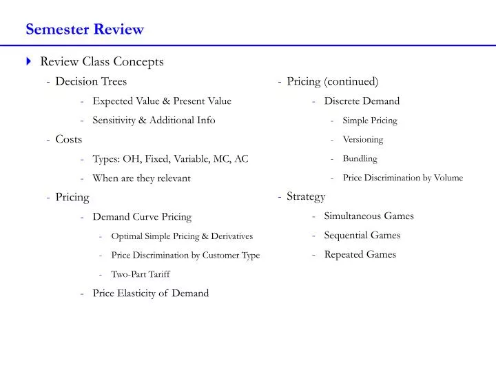
Semester Review • Review Class Concepts • Decision Trees • Expected Value & Present Value • Sensitivity & Additional Info • Costs • Types: OH, Fixed, Variable, MC, AC • When are they relevant • Pricing • Demand Curve Pricing • Optimal Simple Pricing & Derivatives • Price Discrimination by Customer Type • Two-Part Tariff • Price Elasticity of Demand • Pricing (continued) • Discrete Demand • Simple Pricing • Versioning • Bundling • Price Discrimination by Volume • Strategy • Simultaneous Games • Sequential Games • Repeated Games
Class Concepts – Decision Trees • Setting Up Decision Trees • Things to Remember • What decisions do you need to make, and in what order? • Ignore Sunk Costs - What have you already paid for or committed to purchasing? • Remember to include (or mentally consider) the option of exiting the market at the root node and subsequent decision nodes. Once you have the results of R&D or additional information, it may no longer make sense to proceed. • Opportunity Costs - What are your other options? Subtract opportunity costs from your payouts • Values at the Leaves • Calculating the payouts at each leaves involves calculating all the revenues and costs (ignoring sunk costs, and subtracting opportunity costs) that occurred in order to arrive at that outcome. • In some cases, calculating these values may require a present value calculation if revenue or costs are incurred over time (as they did in your midterm…)
Class Concepts – Calculating Present Value • How much would you pay to receive $100 in 1 year? • Discounting: C/(1+r)n • $100/(1+0.1)1 = $90.91 • How much would you pay to receive $100 a year forever if your first payment is one year from now. What if your first payment were today? • Perpetuity formula for payments beginning in 1 year: C/r • $100/0.10 = $1,000 • Perpetuity formula for payments beginning today: C + C/r • $100 + $1,000 = $1100 • Memorize this!
Class Concepts –Decision Trees • Backward Induction • Start from the “leaves” of the tree and work toward the “root” • This is counterintuitive, but since each decision/chance node is independent of the others, we can start by solving the simplest decision, and work back toward the more complicated one we started with • Decision Nodes • Choose the best of the options • Chance Nodes • Find the expected value of the outcomes EV = 5*0.4 + -10*0.6 EV = 2 – 6 EV = -4
Class Concepts – Decision Trees • Setting Up Decision Trees • Value of Information • If you are asked to consider the value of information, try purchasing the information first, as it is likely to be most valuable at that point. • Place a chance-node as your first node • The probabilities of receiving different information from your “expert” or “research” will mirror the probabilities of the same outcomes before you had the information. For instance, if you have a 30% probability of rain and 70% probability of sun. An expert will tell you with certainty that “it will rain” 30% of the time, and “it will be sunny” 70% of the time. • After you receive positive information, you will be more likely to continue with production. • After you receive negative information (like small market potential), you will be less likely to continue with production, and you should add a decision-node for exiting the market. • Sensitivity – on a cost/revenue value or a probability • Ask the question: What am I conducting sensitivity on? What is the next best decision—Is it choosing a different strategy or exiting the market entirely? • Sensitivity on a Cost or Revenue Value • Replace the cost or revenue with a variable across the entire tree • Use backward induction to recalculate the values at each node • Determine for what values of the variable your decision changes • Sensitivity on a Probability (for Chance Nodes) • Replace the probability with a variable, p, and use (1-p) for the probability of the other option at the chance node. • Again, use backward induction to recalculate the values at each node • Determine for what values of p, your decision changes.
Class Concepts – Costs • Costs • Sunk Cost • Costs that are already paid or must be paid even if we decide not to produce • Opportunity Cost • Value of the best (highest-value) foregone alternate use of a resource • Overhead Costs (or Fixed Costs) • Costs that must be paid no matter how much we decide to produce • Variable Costs (or Direct Costs) • Costs that are a function of how much we decide to produce. (i.e. cost of labor and materials) • Marginal Costs • Change in total cost of producing one more unit. This may be higher than variable costs if producing one more unit requires incurring fixed costs. • Average Cost • Total cost divided by number of units produced. • Increasing Returns to Scale AC declines when more units are produced • Constant Returns to Scale AC stays the same regardless of units produced • Decreasing Returns to Scale AC increases when more units are produced
Class Concepts – Pricing – Demand Curve Pricing • Demand Curve Pricing • During class we’ve seen three kinds of pricing (simple and advanced) that involve demand curves. They are: • Optimal Simple Pricing – Set one price for all customers • One demand curve, one customer type • Price Discrimination by Customer Type – Charge different prices to different customer types • Two demand curves, two customer types • Two-Part Tariff – Charge a fixed fee for the right to purchase units, and set a unit cost • One or two customer types and demand curves
Class Concepts – Demand Curve Pricing – Simple Pricing • Steps for Solving an Optimal Simple Pricing Problem • 1) Identify your total cost function (TC) and inverse demand function • Find the inverse demand function by finding the demand function and solving for P • 2) Solve for marginal cost (MC) and marginal revenue (MR) by taking derivatives • 3) Set MC = MR, and solve for Q* • 4) Insert Q* into your inverse demand function and solve for P* • 5) Check that you are profitable: • Profit = Total Revenue – Total Cost • π = P* x Q* – TC ≥ 0 • ** Be sure to do the last step! Optimal Simple Pricing helps you figure out the most profit you can make from selling a good, given available demand. Is that optimal price high enough to cover your fixed costs?
Class Concepts – Calculating a Derivative • What is a derivative • The slope! • How to take a derivative • Total Cost = Ax2 + Bx + C where A, B, and C are coefficients. • Derivative of Total Cost = Marginal Cost = 2Ax + B • General Formula • Axn = nAxn-1 • Simple Rules to follow • You can take the derivative of terms that are added together [i.e. the derivative of x2 + 2x = 2x + 2] • Multiplication between terms makes taking derivatives more complicated [i.e. (x + 2)(x + 1)], so multiply out first [derivative of x2 + 3x + 2 = 2x + 3]
Class Concepts – Price Customization by Customer Type • Price Customization by Customer Type • Sell your product to different customer types at different prices • How to use Price Customization by Customer Type • If, you have two identifiable customer types with two different demand curves then: • Use Simple Pricing, Steps 1-3 for each customer type • If you have two unknowns in two equations, use algebra to solve for Q*1 and Q*2 • Follow Simple Pricing, Steps 4-5 for each customer type • Other Considerations • Arbitrage?: Since you are charging different prices to different customers, think about the potential problems with arbitrage between customers in different groups • Better than simple pricing?: Always
Class Concepts – Two-Part Tariff with One Customer Type • Two-Part Tariff with One Customer Type • Charge a “Fixed Fee” for the right to buy units • Then sell each unit at a set “Unit Price” • How to use the Two-Part Tariff with One Customer Type • 1) Set the “Unit Price” equal to the Marginal Cost (MC) of producing a unit • 2) Set the “Fixed Fee” equal to the Consumer Surplus (CS) when selling at Marginal Cost (MC) Find the area of the triangle • If demand curve is linear: • Set the Inverse Demand Curve = MC Solve for QMC • Area of CS = ½*(Constant from Inverse Demand Curve – MC)* QMC • Requirements for using Two-Part Tariff • This pricing method works best when all buyers have the same demand, and may become less valuable (and more complicated) with more demand types • Arbitrage?: No, you are not charging different prices to different customers • Better than simple pricing?: Always with one type of customer
Class Concepts – Two-Part Tariff with Two Customer Types • Two-Part Tariff with Two Customer Types • Charge a “Fixed Fee” for the right to buy units • Then sell each unit at a set “Unit Price” • How to use the Two-Part Tariff with Two Customer Types • You Need: • Number of High Type, Low Type Customers (NHT, NLT), these will be numbers • Demand for High Type, Low Type Customers, these will be functions • Total Cost (may be based on number of customers and/or number of units sold), this will be a function of the number of customers & number of units • Follow the steps on the following slide:
Class Concepts – Two-Part Tariff with Two Customer Types • How to use the Two-Part Tariff with Two Customer Types (cont.) • How many units will all the low-type customers buy? How many units will all the high-type customers buy? • High Type Units Purchased = # of High Type Customers*(High Type Demand Function) • Low Type Units Purchased = # of Low Type Customers*(Low Type Demand Function) • If the demand function for low-type customers is Q = 10 – P and there are 10,000 customers: • For an unknown price P, each customer will demand (10-P) units. • 10,000 customers will purchase 10-P units • So (100,000 – 10,000P) units will be sold to low-type customers
Class Concepts – Two-Part Tariff with Two Customer Types • How to use the Two-Part Tariff with Two Customer Types (cont.) • There are two types of Revenues: Fixed Fee Revenue & Unit Price Revenue • Use the quantities calculated above to calculate Unit Revenue: • Unit Revenue = Q x P = [High Type Units Purchased + Low Type Units Purchased] x P • Fixed Fee Revenue is based on the consumer surplus of the Low Type Customer. You will collect the fixed fee from both customer types. • Fixed Fee = ½*(Choke Price for Low Type Customer – P)*(Low Type Demand Curve) • Fixed Fee Revenue = Fixed Fee* (# of High Types + # of Low Types) • The demand function for low-type customers is Q = 10 – P, there are 10,000 customers, and these customers will purchase (100,000 – 10,000P) units • Unit Revenue for Low-Type Customers = (100,000 – 10,000P)*P = 100,000P – 10,000P2 • The choke price is where customers will buy zero units. For low type customers, this value is $10. • Fixed Fee = 1/2 *(10 – P)*(10-P) = 1/2 *(100 – 20P + P2) • For total fixed fee revenue, multiply this by the number of both customer types
Class Concepts – Two-Part Tariff with Two Customer Types • How to use the Two-Part Tariff with Two Customer Types (cont.) • Costs can be based on “# of customers” and “# of units purchased” • Costs = Cost for Number of Customers + Cost for Quantity • Costs = Cost/Customer*(# of High Type Customers + # of Low Type Customers) + MC*(High Type Quantity + Low Type Quantity) • The demand function for low-type customers is Q = 10 – P, there are 10,000 customers, and these customers will purchase (100,000 – 10,000P) units. Marginal cost per unit is 2. There is no customer cost. • Cost = 2*(100,000 – 10,000P) = 200,000 – 20,000P
Class Concepts – Two-Part Tariff with Two Customer Types • How to use the Two-Part Tariff with Two Customer Types (cont.) • Profit = Revenues – Costs • Set the Derivative of Profits = 0 • Solve for optimal P! • Requirements for using Two-Part Tariff with Two Customer Types • One customer type must demand more than the other customer type at every price • Always check to see if you could make more by just selling to the high type! • This was key for one of your homework problems!
Class Concepts – Price Elasticity of Demand • Price Elasticity of Demand
Class Concepts – Price Elasticity of Demand • Definition General Definition Exact Definition • Use the general definition to solve for the elasticity between two sets of known prices and quantities • Use the exact definition to solve for the elasticity at a specific point. You need the demand function and the price.
Class Concepts – Pricing with Discrete Demand • Discrete Demand • We have seen three types of advanced pricing methods that use discrete demand: • Versioning • Bundling • Price Discrimination by Volume • Always compare these discrete methods to simple pricing • Marginal Cost = 1 • Price Book A at $14 for profit of $13 ($14x1 - $1x1 = $13) • Instead of pricing at $7 for profit of $12 ($7x 2 - $1x2 = $12) • Price Book B at $11 for profit of $20 ($11x2 - $1x2 = $20) • Instead of pricing at $16 for profit of $15 ($16x1 - $1x1 = $15)
Class Concepts – Versioning • Versioning • Sell two versions of the same products (usually high and low quality) to customers with different preferences for the product versions. • How to use Versioning • 1) Price the low type product at the low type customer willingness to pay • 2) Price the high type product at the high type customer’s willingness to pay less the consumer surplus he/she receives from buying the low type product • 3) Compare the profit of selling to the high and low type customer with selling to just the high type customer. Choose the strategy that produces the highest profits. • Requirements for using Versioning • This pricing method works best when there are two distinct customer groups and everyone agrees which product version is better than the other. • Arbitrage?: No, you are charging one price for each product version. • Better than simple pricing?: Depends on how expensive it is to create two versions
Class Concepts – Bundling • Bundling • Two or more products that can be consumed separately, packaged together and sold at one price • How to use Bundling • Try Simple Pricing • Price each product at the profit maximizing point • Try Pure Bundling • Price the bundle so that it appeals to all consumers and determine profits • Try Mixed Bundling • Create smaller bundles and offer (some) individual products, and calculate profits • Compare profits of each strategy • Requirements for using Bundling • This pricing method works best when there are two or more customer groups with strong willingness to pay for one product and weaker willingness to pay for the other. • Arbitrage?: Yes, think about how to prevent consumers from unbundling & reselling. • Better than simple pricing?: Depends on how correlated demand is among customers
Class Concepts – Price Customization by Quantity • Price Customization by Quantity • Sell your product in a small package and a large package to customers with different volume preferences • How to use Price Customization by Quantity • Choose the size of the Large Package: For the volume preferring group, find the highest volume for which the consumer Marginal Benefit (MB) is higher than MC • Try all possible smaller sizes for the Small Package. • Set the price of the Small Package equal to the low volume preferring group WTP • Set the price of the Large Package equal to the high volume preferring group WTP less the consumer surplus for purchasing the Small Package (or the consumer surplus for purchasing multiple Small Packages). • Calculate the profit when combining each possible Small Package with the chosen large package and choose the Small Package that maximizes profit • Check the profitability of only the Large Package to the volume preferring group, and choose the more profitable option. • Other Considerations • Arbitrage?: There are definite arbitrage opportunities. Be sure to consider whether they are a problem. • Better than simple pricing?: Not necessarily. Check to be sure!
Class Concepts – Sequential Games • Sequential Games • Decision Trees (yes, they’re back again…) • Two Payoffs: One for you, one for your opponent • Use Backward Induction to solve • Start with the outermost branches and work your way back to the root of the tree • Be careful with payouts. Now there are two to keep track of! • Remember to check which party (you or your opponent) is making the decision at each node • Key Terms • Hold Up – After one party incurs a relationship-specific sunk cost, the other party tries to renegotiate the terms. Fear of holdup can prevent deals from occurring. Reputation (for not holding up or not giving in to blackmail) can make deals possible for relationships with repeat interactions. • Entry Deterrence – An incumbent often cannot credibly claim it will fight a new entrant (since payoffs will be better without a price war). To make this empty threat credible, the incumbent can preemptively making a fixed cost investment (such as building overcapacity) that commits the incumbent to fighting. This strategic commitment to fighting will make it unprofitable for new players to consider entry.
Class Concepts – Simultaneous Games • Simultaneous Games • Two parties with perfect information about the economic value of each outcome to themselves and their opponents. • To Solve: • Look for dominant strategies. • If you find one (or two), determine the equilibrium outcome. • If you don’t find any, continue with the next steps to look for Nash equilibrium(s). • Look for dominated strategies and remove (repeat until there are none remaining) • From the remaining strategies, find all outcomes that neither player would want to deviate from. • Key Terms • Equilibrium – An outcome where neither player could change their strategy to earn a better payoff (holding their opponent’s choice constant). The strategies of both parties and the outcome are the solution to the game • Best Response to a strategy is the choice that maximizes a player’s payoff, given that the other player is using that strategy. At equilibrium, both players chosen strategies are best responses. • Dominant Strategy – Maximizes payoffs regardless of what the other player does (the same strategy is the best response to all possible choices of the other player) • Dominated Strategy – Not a best response to any possible strategy of the other player
Class Concepts – Auctions • Auctions • One-time auction for a single item • English Auction – Ascending bid auction. The item goes to the last party to bid. • Strategy: When to drop out What is your WTP? • Dutch Auction – Descending bid auction. The item goes to the first party to bid. • Strategy: When to start bidding What is your WTP? • First-Price Sealed Bid – All interested parties submit a price. The item goes to the party with the highest bid, at the price he/she submitted. • Strategy: What price to submit Survey the competition • Second-Price Sealed Bid – All interested parties submit a price. The item goes to the party with the highest bid, at the price of the second highest bid submitted. • Strategy: What price to submit Survey the competition
Class Concepts – Repeated Games • Repeated Games • Repeated Games are those with simultaneous decisions over an infinite number of interactions or no known ending point. • Games with simultaneous decisions and a finite number of interactions are sequential games. They should be solved using backward induction, and not the strategies discussed here. • Strategies for Repeated Games • Goal: Sustain price moderation (and higher payoffs) to both firms, even though this is not an equilibrium solution to the simultaneous game • Grim Strategy – Price at the optimal industry price. If an opponent cheats and prices lower, punish them by pricing at marginal cost forever. • t-period Trigger Strategy – Price at the optimal industry price. If an opponent cheats and prices lower, price at marginal cost for the next “t” periods. Then return to the optimal industry price. • Tit for Tat Strategy – Price at the optimal industry price. If an opponent cheats and prices lower, then price at marginal cost in the subsequent period.