Download
1 / 27
270 likes | 477 Views
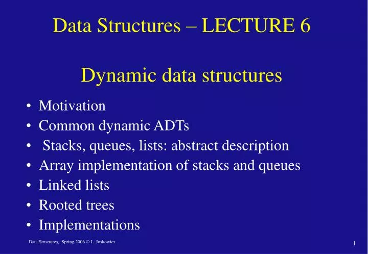
Data Structures – LECTURE 6 Dynamic data structures. Motivation Common dynamic ADTs Stacks, queues, lists: abstract description Array implementation of stacks and queues Linked lists Rooted trees Implementations. 2. 0. 5. 3. 4. 1. 2. 4. 3. 1. 0. 5. Motivation (1).

E N D
Data Structures – LECTURE 6 Dynamic data structures • Motivation • Common dynamic ADTs • Stacks, queues, lists: abstract description • Array implementation of stacks and queues • Linked lists • Rooted trees • Implementations
2 0 5 3 4 1 2 4 3 1 0 5 Motivation (1) • So far, we have dealt with one type of data structure: an array. Its length does not change, so it is a static data structure. This either requires knowing the length ahead of time or waste space. • In many cases, we would like to have a dynamic data structure whose length changes according to computational needs • For this, we need a scheme that allows us to store elements in physically different order.
Motivation (2) • Examples of operations: • Insert(S, k): Insert a new element • Delete(S, k): Delete an existing element • Min(S), Max(S): Find the element with the maximum/minimum value • Successor(S,x), Predecessor(S,x): Find the next/previous element • At least one of these operations is usually expensive (takes O(n) time). Can we do better?
Abstract Data Types –ADT • An abstract data type is a collection of formal specifications of data-storing entities with a well designed set of operations. • The set of operations defined with the ADT specification are the operations it “supports”. • What is the difference between a data structure (or a class of objects) and an ADT? The data structure or class is an implementation of the ADT to be run on a specific computer and operating system. Think of it as an abstract JAVA class. The course emphasis is on ADTs.
Common dynamic ADTs • Stacks, queues, and lists • Nodes and pointers • Linked lists • Trees: rooted trees, binary search trees, red-black trees, AVL-trees, etc. • Heaps and priority queues • Hash tables
Stacks -- מחסנית • A stack S is a linear sequence of elements to which elements x can only be inserted and deleted from the head of the list in the order they appear. • A stack implements the Last-In-First-Out (LIFO) policy. • The stack operations are: • Stack-Empty(S) • Pop(S) • Push(S,x) • A stack S is a linear sequence of elements to which elements x can only be inserted and deleted from the head of the list in the order they appear. • A stack implements the Last-In-First-Out (LIFO) policy. • The stack operations are: • Stack-Empty(S) • Pop(S) • Push(S,x) Push Pop 2 head 0 1 5 null
2 0 2 3 0 1 Queues -- תור • A queue Q is a linear sequence of elements to which elements are inserted at the end and deleted from the beginning. • A queue implements the First-In-First-Out (FIFO) policy. • The queue operations are: • Queue-Empty(Q) • EnQueue(Q, x) • DeQueue(Q) DeQueue EnQueue head tail
2 0 2 3 0 1 Lists -- רשימות • A list L is a linear sequence of elements. • The first element of the list is the head and the last is the tail. When both are null, the list is empty • Each element has a predecessor and a successor • The list operations are: • Successor(L,x), Predecessor(L,x) • List-Insert(L,x) • List-Delete(L,x) • List-Search(L,k) head x tail
Implementing stacks and queues • Array implementation • use an array A of n elements A[i], where n is the maximum number of elements expected. • Top(A), Head(A), and Tail(A) are array indices • Stack and queue operations involve index manipulation • Lists are not efficiently implemented with arrays • Linked list • Create objects for elements as they appear • Do not have to know the maximum size in advance • Manipulate pointers
Stacks: array implementation • Push(S, x) • if top[S] = length[S] • thenerror “overflow” • top[S] top[S] + 1 • S[top[S]] x 1 5 2 3 top Direction of insertion • Pop(S) • if top[S] = 0 • thenerror “underflow” • else top[S] top[S] – 1 • return S[top[S] +1] • Stack-Empty(S) • if top[S] = 0 • thenreturn true • elsereturn false
Queues: array implementation • Dequeue(Q) • x Q[head[Q]] • if head[Q] = length[Q] • then head[Q] 1 • else head[Q] (head[Q]+1)mod n • returnx 0 1 5 2 3 head tail • Enqueue(Q, x) • Q[tail[Q]] x • if tail[Q] = length[Q] • then tail[Q] x • else tail[Q] (tail[Q]+1)mod n Boundary conditions omitted
head tail … a1 a2 an a3 null null Linked Lists -- רשימות מקושרות • The physical and logical order of elements need not be the same; instead, use pointers to indicate where the next (previous) element is. • By manipulating the pointers, we can insert and delete elements without having to move all the others! Lists can be signly or doubly linked.
Nodes and pointers • A node is an object that holds the data, a pointer to the next node and (optionally), a pointer to the next node. If there is no next node, the pointer is to “null” • A pointer indicates the memory address of a node • Nodes usually occupy constant space: Θ(1) key • Class ListNode { • Object key; • Object data; • ListNode next; • ListNode prev; • } data next prev
q a1 a3 a2 a1 a2 a3 next[q]r next[p] q Example: Insertion Insertion of a new node q between successive nodes p and r: p r p r
p r p q r q a1 a2 a3 a1 a3 a2 next[p]r next[q]null null Example: Deletion Deletion of a node q between previous node p and successor node r
Linked lists operations • List-Search(L, k) • x head[L] • whilex ≠ null and key[x]≠k • do x next[x] • return x • List-Insert(L, x) • next[x] head[L] • if head[L]≠ null • then prev[head[L]] x • head[L] x • prev[x] null • List-Delete(L, x) • if prev[L]≠ null • then next[prev[x]] next[x] • else head[L] next[x] • if next[L]≠ null • then prev[next[x]] prev[x]
a1 a2 a4 a3 Example: linked list operations x head tail null null Circular lists: connect first and last elements!
Rooted trees • A rooted tree T is an ADT in which elements are ordered in a tree-like structure. • A tree consists of nodes, which hold elements, and edges, which show relations between two nodes. • There are three types of nodes: a root, internal nodes, leaf • The tree structure is: • Connected: there is an edge path from the root to any other node • No cycles: there is only one path from the root to a node • Each node except the root has a single ancestor • Leaves have no outgoing edges • Internal nodes have one or more out-going edges (= 2 binary)
A B D C H I G E F J N K L M Rooted tree: example 0 1 2 3
Trees terminology • Internal nodes have a parent and one or more children. • Nodes on the same level are siblings (children of the same parent) • Ancestor/descendent relationships – recursive definition of parent and children. • Degree of a node: number of children • Path: a sequence of nodes n1, n2, … ,nk such that ni is a parent of ni+1. The path length is k. • Tree height: length of the longest path from a root to a leaf. • Node depth: length of the path from the root to the node.
Binary trees • A binary tree T is a tree whose root and internal nodes have at most two children. • Recursively: a binary tree is a tree that either contains no nodes or consists of a root node, and two sub-trees (left and right) each of which is also a binary tree.
A B C D E F G Binary tree: example A B C D E F G The order matters!!
A A B C B C D E D E F G F G Full and complete trees • Full binary tree: each node has either degree 0 (a leaf) or 2 exactly two non-empty children. • Complete binary tree: a full binary tree in which all leaves have the same depth. Full Complete
Properties of binary trees • How many leaf nodes does a complete binary tree of height d have? 2d • What is the number of internal nodes in such a tree? 1+2+4+…+2d–1 = 2d –1(less than half!) • What is the total number of nodes? 1+2+4+…+2d = 2d+1–1 • How tall can a full/complete binary tree with n leaf nodes be? (n –1)/2 2d+1 –1= n log (n+1) –1 ≤log (n)
level 0 A 1 B C D E 2 2 F G Array implementation of binary trees 1 2d elements at level d 2 3 4 5 6 7 Complete tree: parent(i) = floor(i/2) left-child(i) = 2i right-child(i) = 2i +1 1 2 3 4 56 7 A B C D E F G 20 21 22
Linked list implementation of binary trees root(T) A • Each node contains • the data and three • pointers: • ancestor(node) • left-child(node) • right-child(node) B C D E F G data H
G F H I J Linked list implementation of general trees root(T) A • Left-child/right sibling • representation • Each node contains • the data and three • pointers: • ancestor(node) • left-child(node) • right-sibling(node) B C D D E K