Introduction to Polygons

1. Introduction to Polygons • Different types of Polygons • Simple Convex • Simple Concave • Non-simple : self-intersecting • With holes Convex Concave Self-intersecting

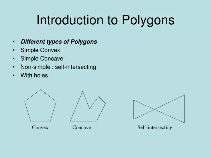
2. Introduction to Polygons • Convex A region S is convex iff for any x1 and x2 in S, the straight line segment connecting x1 and x2 is also contained in S. The convex hull of an object S is the smallest H such that S

3. Scan Line Polygon Fill Algorithms • A standard output primitive in general graphics package is a solid color or patterned polygon area: • There are two basic approaches to filling on raster systems. • Determine overlap Intervals for scan lines that cross that area. • Start from a given interior point and paint outward from this point until we encounter the boundary • The first approach is mostly used in general graphics packages, however second approach is used in applications having complex boundaries and interactive painting systems Xk+1,yk+1 Scan Line yk +1 Scan Line yk Xk , yk

4. Seed Fill Algorithm • These algorithms assume that at least one pixel interior to a polygon or region is known • Regions maybe interior or boundary defined Interior-defined region Interior-defined region

5. A Simple Seed Fill Algorithm Push the seed pixel onto the stack While the stack is not empty Pop a pixel from the stack Set the pixel to the required value For each of the 4 connected pixels Adjacent to the current pixel, check if it is a boundary pixel or if it has already been set to the required value. In either case ignore it. Otherwise push it onto the stack • The algorithm can be implemented using 8 connected pixels • It also works with holes in the polygons

6. Scan Line Polygon Fill Algorithm 10 14 18 24 Interior pixels along a scan line passing through a polygon area • For each scan line crossing a polygon are then sorted from left to right, and the corresponding frame buffer positions between each intersection pair are set to the specified color. • These intersection points are then sorted from left to right , and the corresponding frame buffer positions between each intersection pair are set to specified color

7. Scan Line Polygon Fill Algorithm • In the given example ( previous slide) , four pixel intersections define stretches from x=10 to x=14 and x=18 to x=24 • Some scan-Line intersections at polygon vertices require special handling: • A scan Line passing through a vertex intersects two polygon edges at that position, adding two points to the list of intersections for the scan Line • In the given example , scan Line y intersects five polygon edges and the scan Line y‘ intersects 4 edges although it also passes through a vertex • y‘ correctly identifies internal pixel spans ,but need some extra processing

8. Scan line Polygon Fill Algorithm • One way to resolve this is also to shorten some polygon edges to split those vertices that should be counted as one intersection • When the end point y coordinates of the two edges are increasing , the y value of the upper endpoint for the current edge is decreased by 1 • When the endpoint y values are monotonically decreasing, we decrease the y coordinate of the upper endpoint of the edge following the current edge

9. Scan Line Polygon Fill Algorithm (a) (b) Adjusting endpoint values for a polygon, as we process edges in order around the polygon perimeter. The edge currently being processed is indicated as a solid like. In (a), the y coordinate of the upper endpoint of the current edge id decreased by 1. In (b), the y coordinate of the upper end point of the next edge is decreased by 1

10. Scan Line Polygon Fill Algorithm • The topological difference between scan Line y and scan Line y'

11. The topological difference between scan line y and scan line y’ is … • For Scan line y, the two intersecting edges sharing a vertex are on opposite sides of the scan line …! • But for scan line y’, the two intersecting edges are both above the scan line • Thu, the vertices that require additional processing are those that have connecting edges on opposite sides of scan line. • We can identify these vertices by tracing around the polygon boundary either in clock-wise or anti-clockwise order and observing the relative changes in vertex y coordinates as we move from one edge to the next. • If the endpoint y values of two consecutive edges monotonically increase or decrease, we need to count the middle vertex as a single intersection point for any scan line passing through that vertex.

12. Otherwise, the shared vertex represents a local extremum (min. or max.) on the polygon boundary, and the two edge intersections with the scan line passing through that vertex can be added to the intersection list Figure 3-36 Intersection points along the scan lines that intersect polygon vertices. Scan line y generates an odd number of intersections, but scan line y generates an even number of intersections that can be paired to identify correctly the interior pixel spans.

13. The scan conversion algorithm works as follows • Intersect each scanline with all edges • Sort intersections in x • Calculate parity of intersections to determine in/out • Fill the “in” pixels • Special cases to be handled: • Horizontal edges should be excluded • For vertices lying on scanlines, • count twice for a change in slope. • Shorten edge by one scanline for no change in slope • Coherence between scanlines tells us that • Edges that intersect scanline y are likely to intersect y + 1 • X changes predictably from scanline y to y + 1

14. We have 2 data structures: Edge Table and Active Edge Table • Traverse Edges to construct an Edge Table • Eliminate horizontal edges • Add edge to linked-list for the scan line corresponding to the lower vertex. • Store the following: • y_upper: last scanline to consider • x_lower: starting x coordinate for edge • 1/m: for incrementing x; compute • Construct Active Edge Table during scan conversion. AEL is a linked list of active edges on the current scanline, y. Each active edge line has the following information • y_upper: last scanline to consider • x_lower: edge’s intersection with current y • 1/m: x increment • The active edges are kept sorted by x

15. Algorithm • Set y to the smallest y coordinate that has an entry in the ET; i.e, y for the first nonempty bucket. • Initialize the AET to be empty. • Repeat until the AET and ET are empty: • 3.1 Move from ET bucket y to the AET those edges whose y_min = y (entering edges). • 3.2 Remove from the AET those entries for which y = y_max (edges not involved in the next scanline), the sort the AET on x (made easier because ET is presorted). • 3.3 Fill in desired pixel values on scanline y by using pairs of x coordinates from AET. • 3.4 Increment y by 1 (to the coordinate of the next scanline). • 3.5 For each nonvertical edge remaining in the AET, update x for the new y. • Extensions: • Multiple overlapping polygons – priorities • Color, patterns Z for visibility