Download
1 / 109
1.09k likes | 1.1k Views
452 NWP 2016. Major Steps in the Forecast Process. Data Collection Quality Control Data Assimilation Model Integration Post Processing of Model Forecasts Human Interpretation (sometimes) Product and graphics generation. Data Collection.

E N D
Major Steps in the Forecast Process • Data Collection • Quality Control • Data Assimilation • Model Integration • Post Processing of Model Forecasts • Human Interpretation (sometimes) • Product and graphics generation
Data Collection • Weather is observed throughout the world and the data is distributed in real time. • Many types of data and networks, including: • Surface observations from many sources • Radiosondes and radar profilers • Fixed and drifting buoys • Ship observations • Aircraft observations • Satellite soundings • Cloud and water vapor track winds • Radar and satellite imagery
Weather Satellites Are Now 99% of the Data Assets Used for NWP • Geostationary Satellites: Imagery, soundings, cloud and water vapor winds • Polar Orbiter Satellites: Imagery, soundings, many wavelengths • RO (GPS) satellites • Scatterometers • Active radars in space (GPM)
Quality Control • Automated algorithms and manual intervention to detect, correct, and remove errors in observed data. • Examples: • Range check • Buddy check • Comparison to first guess fields from previous model run • Hydrostatic and vertical consistency checks for soundings. • A very important issue for a forecaster--sometimes good data is rejected and vice versa.
Eta 48 hr SLP Forecast valid 00 UTC 3 March 1999 3 March 1999: Forecast a snowstorm … got a windstorm instead
Pacific Analysis At 4 PM 18 November 2003 Bad Observation
Forecaster Involvement • A good forecast is on the lookout for NWP systems rejecting bad data, particularly in data sparse areas. • Quality control systems can allow models to go off to never never land. • Less of a problem today due to satellite data everywhere.
Objective Analysis/Data Assimilation • Observations are scattered in three dimensions • Numerical weather models are generally solved on a three-dimensional grid • Need to interpolate observations to grid points and to ensure that the various fields are consistent and physically plausible (e.g., most of the atmosphere in hydrostatic and gradient wind balance).
Objective Analysis • Interpolation of observational data to either a grid (most often!) or some basis function (e.g., spectral components) • Typically iterative (done in several passes)
Objective Analysis/Data Assimilation • Often starts with a “first guess”, usually the gridded forecast from an earlier run (frequently a run starting 6 hr earlier) • This first guess is then modified by the observations. • Adjustments are made to insure proper balance. • Often iterative
3DVAR: 3D Variational Data Assimilation • Used by the National Weather Service today for the GFS and NAM (called GSI) • Tries to create an analysis that minimizes a cost function dependent on the difference between the analysis and (1) first guess and (2) observations • Does this at a single time.
4DVAR: Four Dimension Variational Data Assimilation • Tries to optimize analyses at MULTIPLE TIMES • Tries to duplicate the observed evolution over time as well as the situation at initialization time. • Uses the model itself as a data assimilation too.
4DVAR Components • Full non-linear model • Tangent linear version of the full model (linearized version of the forecast model) • Adjoint of the tangent linear model -which allows one to integrate the model backwards. Tells sensitivity of final state to the initial state.
4DVAR • Typical runs the model back and forth during an initialization period (6-12 hr), roughly ten times. • Substantial computational cost. • Need to have adjoint and TL version of the model. • Currently used by ECMWF, CMC, UKMET, and US Navy. NOT NCEP.
Many of the next generation data assimilation approaches are ensemble based • Example: the Ensemble Kalman Filter (EnKF)
Mesoscale Covariances 12 Z January 24, 2004 Camano Island Radar |V950|-qr covariance
Surface Pressure Covariance Land Ocean
An Attractive Option: EnKF Temperature observation 3DVAR EnKF
Hybrid Data Assimilation: Now Used in GFS • Uses both 3DVAR and EnkF • Uses EnkF covariances from GFS ensemble in 3DVAR.
Next Advance ENVAR • Use temporal covariances to spread impact of observations over TIME. • Will go operational NEXT WEEK. • Has some of the properties of 4DVAR (adjusts model evolution)
Vertical Coordinate Systems • Originally p and z: but they had a problem…BC when the grid hit terrain! • Then eta, sigma p and sigma z, theta • Increasingly use of hybrids– e.g., sigma-theta
Why Nesting? • Could run a model over the whole globe, but that would require large amounts of computational resource, particularly if done at high resolution. • Alternative is to only use high resolution where you need it…nesting is one approach. • In nesting, a small higher resolution domain is embedded with a larger, lower-resolution domain.
Nesting • Can be one-way or two way. • In the future, there will be adaptive nests that will put more resolution where it is needed. • And instead of rectangular grids, other shapes can be used.
Next Generation Global Models Under Development! • Will use different geometries
Model Integration: Numerical Weather Prediction • The initialization is used as the starting point for the atmospheric simulation. • Numerical models consist of the basic dynamical equations (“primitive equations”) and physical parameterizations.
“Primitive” Equations • 3 Equations of Motion: Newton’s Second Law • First Law of Thermodynamics • Conservation of mass • Perfect Gas Law • Conservation of water With sufficient data for initialization and a mean to integrate these equations, numerical weather prediction is possible. Example: Newton’s Second Law: F = ma