Download
1 / 36
360 likes | 450 Views
Presentation to the Swiss CFA Society Geneva, May 11, 2010 Zurich, May 19, 2010. Portfolio Design. Renato Staub May 2010. www.singerLLC.com. Objectives. Here, we deal with the expectation based market allocation.

E N D
Presentation to the Swiss CFA SocietyGeneva, May 11, 2010Zurich, May 19, 2010 Portfolio Design Renato Staub May 2010
www.singerLLC.com Objectives • Here, we deal with the expectation based market allocation. • In classical portfolio management, this is referenced as ‘active’ allocation. • We want to improve the asset allocation (AA) design process. In particular, we are: • Recognizing that history may be a questionable guide to the future by using historical parameters to simulate the opportunity • Calibrating the amount of risk taken, given the opportunity, in order to reasonably expect to achieve the risk budget over time • Providing a framework for checking the consistency across capabilities • Making the investment process more transparent
www.singerLLC.com Concepts • Given the value/price signals over time, we are looking for the • Appropriate expectation based AA strategy • According amount of risk • Composition of this strategy • We combine the following concepts: • Value/Price as based on discounted cash flow models • Random walks • Mean reversion • Information analysis • We integrate them in a single framework.
www.singerLLC.com Nature of Asset Allocation • There are concepts that do not entail imbalances, e.g. Black-Scholes. • That is, the market goes up or down with equal probability. • By contrast, AA assumes that markets • Deviate from their intrinsic value • Revert in the long run. • Without mean reversion, AA cannot add value. • Hence…
www.singerLLC.com … we want to ride this wave!
www.singerLLC.com Eye-Catcher • We simulate • Value/Price of a mean reverting market • Monthly over 1000 years • The market’s average return equals 8.5% (f1). • The upper chart entails all • Under-valuations >20% and <30% • The lower chart shows the subsequent • Ann. 3-year returns (f2). • We observe: f2 >> f1. • Without mean reversion, f2 would equal f1.
www.singerLLC.com Terminology • We deal with two key inputs, i.e. • A market’s price, P • Its fundamental value, V • P can be observed for liquid markets. • V cannot be observed. It must be estimated by a concept. • We model in log space, i.e. v = log(V) and p = log(P). • The value-price relationship is defined as follows: vp = log(V/P) = log(V) – log(P) = v-p • Assuming that p reverts to v over the duration d, this implies xr = (v-p) / d • xr is the expected return component due to price correction.
www.singerLLC.com Numerical Example • The following parameters are given: • V = 100 (by definition) • P = 80 • d = 3 years • V/P = 100/80 = 1.25 • vp = log(V/P) = v-p = log(100/80) = 0.2231 • xr = (v-p) / d = 0.2231 / 3 = 7.44% • That is, we expect an additional log. return of 7.44% p.a. due to price correction. • However, this is a raw expectation. • Later on, there will be a further modification to xr.
www.singerLLC.com Plan • We simulate the vp evolution over a long time. • We calibrate the simulation such that the resulting • vp span • vp volatility • Reversion time are in line with practical experience. • We infer the information embedded in this process. • We translate this information into a portfolio. • We investigate the portfolio, in particular • Its performance • Other important properties
www.singerLLC.com Process - p • We assume that the price follows a random walk. • The shocks are based on our forward looking covariance matrix. • The market price is shocked proportionally to its size, that is pt+1 = pt + • However, in order to avoid infinite dispersion, we must ensure mean reversion. • To that end, we adjust the equation as follows pt+1 = pt (1-pp) + p • pp is p’s gap sensitivity of mean reversion. • From time series analysis, we know • < 0 The process is stationary • >= 0 The process is non-stationary
www.singerLLC.com Process – v • Nobody knows v, and this is why we estimate it. • We assume it to fluctuate around its (unknown) ‘true’ intrinsic value, i.e. vt+1 = vt (1-vv) + v • vv is v’s gap sensitivity of mean reversion. • But in practice, we often review a model in case of a large vp discrepancy. • This applies in particular to markets of low model confidence. • Technically, it means a gap sensitivity of v vs. p, that is vt+1 = vt (1-vv) + (vt-pt) (1-vp) + v = vt+1 = vt (2-vv-vp) - pt (2-vp) + v • We reference this effect as ‘chasing’: the (perceived) value chases the price. • This means a narrowing of vp, i.e. the perceived opportunity becomes smaller.
www.singerLLC.com Process – Combining v and p • Combining v and p, we get vpt+1 = vt (2-vv-vp) - pt (2-pp -vp) + v + p • The next chart is a vp simulation based on monthly data over 1000 years. • Notably, vp is confined to a certain bandwidth - because of mean reversion. • The breadth of the band depends on the input parameters.
www.singerLLC.com Process - Information • As a result of mean reversion, there is a positive correlation between the • Expected return from correction (i.e. the signal) • Observed subsequent return from correction • Hence, we are interested in the correlation between the two, that is R = corr(Ei[xr(i,i+d)], xr(i,i+1)) where xr(i,i+d) is the return from correction between time i and time i+d. • Because of the substantial noise components, this correlation is small. • In other words, our signal, xr, is far from perfect. • We define R = IC = Information Coefficient
www.singerLLC.com Process - Property • Shape Invariance Theorem: vp evolutions with identical b‘s entail identical information. • As an example, the following charts portray two markets. The • Blue market has shock components of 2s. • Red market has shock components of s. • Mean reversion parameters of both markets are identical. • As expected, both ICs inferred from simulation equal 0.118192.
www.singerLLC.com Process - Calibration • The main calibration parameters are the • Volatilities • Mean reversion parameters • The chart to the right shows the percentiles of our simulation based vp distribution. • As a reference, our valuation considered U.S. equity • 60% overvalued in 2000 (techno bubble) • 50% undervalued in 2009 (credit crisis) • The according percentiles relative to the market risks are wider for equity than for bonds. • This is because we set stronger mean reversion for bonds than equity.
www.singerLLC.com FLAM and PAR • The Fundamental Law of Active Management (FLAM) infers: • A portfolio’s information ratio (IR) equals the IC of the comprising markets (i.e. signal projection) times the square root of the number of independent market bets available. *) • The Proportional Allocation Rule (PAR) concludes: • To allocate efficiently, we should allocate proportional to the signal. **) • While • FLAM describes performance • PAR tells us how to achieve it *) Assuming the various markets have identical ICs **) Assuming the signals are uncorrelated and have identical volatilities
www.singerLLC.com PAR – Schematic Example • At time 0 • The price equals p and the value equals v • According to PAR, we buy an amount of (v-p) • Between time 0 and 1 • The price changes by • Hence, the value price discrepancy changes to (v-p-) • At time 1’ • According to PAR, we adjust the quantity by - • Between time 1 and 2 • The price changes by - • We have the quantity (v-p-) at price p • The net gain equals 2
www.singerLLC.com PAR – Schematic Example • The same principle works for two up moves combined with two down moves. • For all four combinations, i.e. • up-up-down-down • up-down-up-down • down-down-up-up • Down-up-down-up • PAR results in a net gain of 22 . • Exposure Theorem: Following PAR at constant volatility, the extra return grows with time. • On the other hand, the size of the extreme vp is irrelevant.
www.singerLLC.com Slide in – Geometrical Representation of Risk • Risk can be depicted by the length of a vector. • And correlation equals the cosine of the angle between two risks. • In the following triangle, the labels mean • Risk of Portfolio 1 (Pf1): s1 • Risk of Portfolio 2 (Pf2): s2 • Correlation between Pf1 and Pf2: cos(j) • Relative Risk (Tracking Error) between Pf1 and Pf2: s1 - s2 s1 s1 - s2 j s2
www.singerLLC.com Signal - Information • We represent both the signal and the observation by vectors. • The more the signal points in the direction of the observation, the better it is. • Hence, a signal’s prediction quality equals its • Projection onto the observation axis • The projection equals the • Correlation between signal and observation • Cosine of angle j • Again, “correlation” and “cosine” are two different labels for the same thing. Signal j Observation Projected Signal
www.singerLLC.com Signal - Modification • xri is the naïve expected extra return for market i • But only its projection will materialize statistically • Hence, we IC-correct it • Further, a return must always be put in relation to its distribution. • Thus, we divide xri by the volatility of market i. • Ultimately, the “true” substance of xri equals xri
www.singerLLC.com Signal - Modification • Assume an equity and a bond market have an si of equal size. • Identical allocation to equity and bonds implies more portfolio risk from equity. • Since PAR assumes identical risks, we must rescale one more time by the risk: • Ultimately, the suggested allocation equals • The portfolio risk is linear in f.
www.singerLLC.com Allocation – Vector Approach • All bets are made vs. cash (only). • That is, in case of cash, C, and two markets, A and B, the vector approach • Bets A vs. C • Bets B vs. C • Does not bet A vs. B • Hence, the set of all bets is a one-dimensional structure. • This is why we call it “Vector Approach”. • The vector approach is mainly a bet of cash vs. the entire market.
www.singerLLC.com Allocation – Matrix Approach (First Scenario) • The matrix approach makes all possible bets, that is, also the bet A vs. B. • The relative risk between A and B is marked in red. • The triangle ABC is positioned such that its corners touch the corresponding iso-vp lines. • As B is more undervalued than A, we go long B vs. A. • Based on the vp differential and the risk geometry, this bet will be of average size. • That is, the bet A vs. B has mainly implications in terms of diversification. VP=20% VP=7% VP=0% B C A
www.singerLLC.com Allocation – Matrix Approach (Second Scenario) • The vp differential between A and B is unchanged. • But A and B are correlated much stronger vs. the first scenario. • Hence, we scale by a smaller risk distance. • As a result, A vs. B is by far the strongest bet. • That is, its implication goes beyond diversification only. • Rather, it is supposed to beef up return. VP=20% VP=7% B VP=0% A C
www.singerLLC.com Signal – Hosting the Matrix Approach • We build the difference between two IC corrected extra returns. • And the risk is the relative risk between the two markets. • That is: • wijis the position based on the relative bet between market i and market j. • The above equation also serves the vector approach, in which case j labels cash.
www.singerLLC.com Simulations – Valuation
www.singerLLC.com Simulations – Matrix Approach
www.singerLLC.com Simulations – Vector Approach Zero
www.singerLLC.com Simulations – Valuation and Suggested Allocation
www.singerLLC.com Allocation - Comparison • Vector approach: • xri and wi have always identical signs. • Cash is a special bucket, as all bets are made vs. cash. • Hence, the cash dispersion is massively larger. • Matrix approach: • xri and wi do not necessarily have identical signs. • Market i may be undervalued but shorted vs. most other markets. • The reason is: it may be less undervalued than other markets. • Cash is a bucket like any other. • Hence, the cash dispersion is much smaller.
www.singerLLC.com Performance - Comparison
www.singerLLC.com Performance - Comparison • Resulting Information Ratios (IR), based on 20 market bets: • Vector Approach: 0.93 • Matrix Approach: 1.48 • Overall, the level of the resulting IR seems (too) high. • This is partially due to the stationarity underlying our framework. • Realistically, that’s the best possible assumption. • However, the high IR is also due to efficient use of information. • Notably, the matrix approach performs much better. • The reason is its better diversification. • The portfolio can be scaled through f to any risk/return level at the given IR.
www.singerLLC.com Summary and Conclusions • We develop a formal allocation process that is • Transparent • Consistent across markets • To that end, we • Calibrate and simulate a mean reverting value/price process • Extract and translate the embedded signals • We present two translation approaches • Vector approach: all market bets are made vs. cash • Matrix approach: there are also bets between markets • The matrix approach performs better, as it is better diversified. • We may deviate from the suggested allocation; the according performance difference is attributed to non-fundamental factors.
www.singerLLC.com Thank you very much for your Attention!
www.singerLLC.com References [1] Grinold, Richard C. and Ronald Kahn. “Active Portfolio Management.” Probus Publications, Chicago, 1995. [2] Hull, Jon C., 1993, Options, Futures, and other Derivatives, Second Edition. Prentice Hall, Englewood Cliffs, NJ. [3] Staub, Renato. “Signal Transformation and Portfolio Construction for Asset Allocation.” Working Paper, UBS Global Asset Management, Sept. 2008. [4] Staub, Renato. “Deploying Alpha: A Strategy to Capture and Leverage the Best Investment Ideas”. A Guide to 130/30 Strategies, Institutional Investor, Summer 2008. [5] Staub, Renato. “Are you about to Handcuff your Information Ratio?” Journal of Asset Management, Vol. 7, No. 5, 2007. [6] Staub, Renato. “Unlocking the Cage”. Journal of Wealth Management, Vol. 8, No. 5, 2006. [7] Staub, Renato. “Deploying Alpha Potential”. UBS Global Asset Management, White Paper, 2006.