Download
1 / 16
160 likes | 237 Views
Statistics Applied to Bioinformatics. Correlation analysis. Mean dot product. The dot product of two vectors is the sum of the pairwise products of the successive terms. The mean dot product is the average of the pairwise products of the successive terms.

E N D
Statistics Applied to Bioinformatics Correlation analysis Jacques van HeldenJacques.van.Helden@ulb.ac.be
Mean dot product • The dot product of two vectors is the sum of the pairwise products of the successive terms. • The mean dot product is the average of the pairwise products of the successive terms. • Positive contributions to the dot product: • When both terms are positive • When both terms are negative • Negative contributions: • When one term is positive, and the other one positive
Converting the dot product into a dissimilarity metrics • The dot product is a similarity metrics. • It can take positive or negative values. • Is is not bounded. • The dot product can be converted into a dissimilarity metrics (dpdab) by substracting it from a constant. • For some applications (clustering), the dissimilarity has to be positive. The constant has thus to be adapted to the data, which is a bit tricky.
Covariance • The covariance is the mean dot product of the centred variables (value minus mean). • The covariance indicates the tendency of two variables to vary in a coordinated way.
Pearson's coefficient of correlation • Pearson’s correlation coefficient corresponds to a standardized covariance • each term of the product is divided by the standard deviation • Whereais the index of an object (e.g. a gene)bis the index of another object (e.g. a gene)iis an index of dimension (e.g. a chip)miis the mean value of the ith dimension • Note the correspondence with z-scores: computing the coefficient of correlation implicitly includes a standardization of each variable. • The correlation is comprised between -1 and 1 • Positive values indicate correlation, negative values anti-correlation.
Correlation distance • Pearson’s correlation coefficient can be converted to a distance metric by a simple operation. • This distance has real values comprised between 0 and 2 • 2 indicates a perfect correlation • 1 indicates that there is no linear correlation between a and b • 0 indicates a perfect anti- correlation
Generalized coefficient of correlation • Pearson correlation can be generalized by using a various types of references raand rb • If the mean values ma and mb are used as references, this gives Pearson’s correlation. • If the references are set to 0, this gives the uncentred coefficient of correlation (see next slide). • Other values can be used if this is justified by some particular knowledge about the data.
Uncentred correlation • A particular case of the generalized correlation is to take the value 0 as reference. • This is called the uncentred correlation. • This choice can be relevant if the object is a gene, and the value 0 represents non-regulation.
Positive and negative contributions to the coefficient of correlation • The contribution of points will be positive or negative depending on their positions relative to the means of the respective dimensions. • In two dimensions • The upper-right and lower-left quadrants (relative to the means) give a positive contribution. • The lower-left and upper-right quadrants (relative to the means) give a positive contribution. - - - + + + - - - + + + - - - + + + 0 + + - + - - + + - + - - my + + - - + - 0 mx
Correlation between the response of yeast transriptome to two carbon sources • We compare the two replicates of the experiment from Gasch, 2000 where ethanol is provided as carbon source. • In grey: all the genes • In blue: 269 genes showing a significant up- or down-regulation in response to at least one carbon source (13 chips). • Most points (and in particular the most distant points) are in the upper-right and lower-left quadrants. • There is a strong positive correlation (cor=0.83).
Correlation between the responses of two carbon sources • We compare the experiments wit ethanol and sucrose as carbon sources, respectively (Gasch, 2000). • In grey: all the genes • In blue: 269 genes showing a significant up- or down-regulation in response to at least one carbon source (13 chips). • Most selected genes show an opposite behaviour : up-regulated in one condition, down-regulated in the other one. • Those genes (upper-left and lower-right quadrants) give negative contributions to the correlation. • Four genes however are strongly down-regulated in both conditions. • Those genes (lower-left quadrant) give positive contributions to the correlation. • The correlation is negative (cor=-0.36), but not as strong as in the previous slide.
Dot product matrix - carbon sources (Gasch 2000) • Data set: 269 genes showing a significant up- or down-regulation in response to carbon sources (Gasch, 2000) • The matrix represents the dot product between each pair of conditions. • Conditions are grouped together (clustered) according to their similarities.
Covariance matrix - carbon sources (Gasch 2000) • Data set: 269 genes showing a significant up- or down-regulation in response to carbon sources (Gasch, 2000) • The matrix represents the covariance between each pair of conditions. • Conditions are grouped together (clustered) according to their similarities. • Note: the diagonal (covariance between a condition and itself) is the variance of each condition.
Correlation matrix - carbon sources (Gasch 2000) • Data set: 269 genes showing a significant up- or down-regulation in response to carbon sources (Gasch, 2000) • The matrix represents the correlation between each pair of conditions. • Conditions are grouped together (clustered) according to their similarities. • Note: the values on the diagonal (correlation between a condition and itself) are always 1.
Euclidian distance - carbon sources (Gasch 2000) • Data set: 269 genes showing a significant up- or down-regulation in response to carbon sources (Gasch, 2000) • The matrix represents the Euclidian distance between each pair of conditions. • Conditions are grouped together (clustered) according to their similarities. • Note: • The values on the diagonal (distance between a condition and itself) are always 0. • The Euclidian distance is always positive, we loose the distinction between correlation and anti-correlation.