Download
1 / 33
330 likes | 426 Views
Geography and Geographical Analysis using the ONS Longitudinal Study. Christopher Marshall & Julian Buxton CeLSIUS. Aims of the Presentation. What is the ONS LS and what data does it contain? What geographical information is in the LS and at what level? What does this allow us to do?

E N D
Geography and Geographical Analysis using the ONS Longitudinal Study Christopher Marshall & Julian Buxton CeLSIUS
Aims of the Presentation • What is the ONS LS and what data does it contain? • What geographical information is in the LS and at what level? • What does this allow us to do? • The strengths and weaknesses of using geographical data in the LS. • Examples of using geographical data in the LS. • The Role of CeLSIUS (Centre for Longitudinal Study Information and User Support).
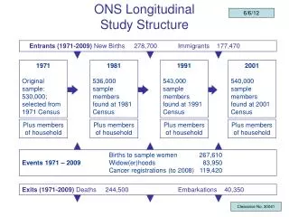
The ONS Longitudinal Study • Census data for individuals with one of four birthdates enumerated at the 1971 Census (c. 1% of population) • Maintained through addition of immigrants and new births with LS birth date • Information from later censuses (1981, 91 & 2001) added and linked to that already there. • Event data including deaths of LS members, cancer registrations, death of spouse, births to female members, and now, under test, the Claimant Count Cohort.
Entrants New Births 214,000 Immigrants 107,000 Births to sample women 201,000 Events 1971 - 2001 Widow(er)hoods 66,000 Cancer registrations70,000 Deaths 189,000 Embarkations 30,000 Study Structure 1971 Original sample: 530,000; selected from 1971 Census 1981 536,000 sample members found at 1981 Census 1991 543,000 sample members found at 1991 Census 2001 545,894 sample members found at 2001 Census Plus members of household Plus members of household Plus members of household Plus members of household 1. Census. High N. 2. Linking 3. Non-members 4. Entrance & Termination 5. Events
Geographical Location of LS Members From Census Information • Based on Address of Usual Residence on Census Day • Visitors flagged prior to 2001 and usually excluded from studies • Fully coded to the Administrative boundaries and also to Health boundaries (e.g. Regional Health Authority)
Main Time Points Available • 1970 from address 1 year ago in 1971 • Census day 1971 (25th/26th April) • 1980 from address 1 year ago in 1981 • Census day 1981 (5th/6th April) • 1990 from address 1 year ago in 1991 • Census day 1991 (21st/22nd April) • 2000 from address 1 year ago in 2001 • Census day 2001 (29th/30th April) • Also possible: 1966 from address 5 years ago 1971 • 1939 (in theory)
What does this allow us to do? • Migration: • Mobility – Geographical & Social Categories • Use existing definitions • Create new analytical definitions • Attach and analyse ecological data • Create new geographies • Analyse specific areas
Social and Geographical Mobility 1971 - Living in NE Social Class: Skilled Non-Manual Tenure: Social Housing 2001 - Living in SE Social Class: Managerial Tenure: Owner Occupier
Use of existing definitions - Geographical • Continuity for 30 years at 1974 geography despite changing boundaries. • Standard Region / Government Office Region • 2001 can be mapped to preceding years and look-up tables can bring earlier geographies forward to 2001 • County and County Districts can be treated similarly.
Use of existing definitions: Geographical (2) • Administrative boundaries • Environmental boundaries • Ecological Deprivation Indices • Area Classifications (Urban / Rural) • Population densities • Small area statistics (Aggregate level variables)
Create new definitions - Geographical • Urban – Rural • Travel to Work • Craig – Webber • Other valid divisions
Create new definitions: Socio-economic • Social Class by Sex • Social Class by Age Group • Working Status – Age Group • Social Class by Tenure
Attach ecological or social data Any data can be attached to individual LS members if it is produced in the form of a look-up table with a valid geographical reference code (e.g. Ward, County District) attached. Air pollution indicators Average rainfall in 10 years Ecological Deprivation indices
Create new geographies It could be that for your specific purpose the Geographies within the LS are inappropriate. Define the geography you want based on LS wards or county districts and this can be attached to LS members and used for analysis. e.g. We have regions but you want to divide each into two or three separate areas not wholly based on counties.
Look at specific areas The purpose of your analysis is to look only at a specific area of the country and compare it with one or two others. Depending on parameters chosen the analysis can run into ‘disclosure control’ restrictions – keep the analysis simple with a limited number of parameters. Analysis at Ward level or below would require aggregation of results, while at county district level, outputs do not usually require aggregation.
Strengths of geographical data in the LS • Consistency over time – 1971, 1981, 1991 all coded to same base (1974 geography). 2001 can be produced on the same base down to county district level with confidence fairly easily. • If necessary earlier data can be brought forward to 2001 by the use of look-up tables.
Strengths of geographical data in the LS • 30 years of continuous follow-up of individuals • 9 Time points (1966 – 2001) • Consistency of geography through this time period.
Strengths of geographical data in the LS • Flexibility of study design • Individual and Area data • Can add data using geographical identifiers (e.g. Carstairs deciles) • High level of detail available for later data.
Weaknesses of geographical data in the LS • While County and County District Codes have remained fairly consistent the Ward codes needed to attach additional data have changed significantly over time. • Data are for England and Wales only • Members who move to Scotland classed as embarkations (migrants)
Weaknesses of geographical data in the LS • Data codings and data detail not consistent. • It is not possible to ‘back transfer’ all geographies. • Ward code history – many changes and manipulations lay traps for the unwary.
Scotland Members in 1971 found with a Scottish NHS number were incorporated into the LS. Events to LS members (e.g. deaths) that occur in Scotland are traced and do get linked to LS members. LS members who migrate to Scotland are treated as Emigrants and this is recorded in the LS. Earlier data remain within the LS.
Disclosure Control Rules Researchers should design their projects such that it would never be possible to identify an individual from the output data generated (Population uniques). Output cell counts of 1 or 2 are considered potentially disclosive (although most 2s will be released to users), and for publication purposes some aggregation of data would be required. Exposure times for single events are a considered a risk and have to be disguised.
Disclosure Control Rules Tables containing data with a mix of any of the following types of variable will be examined more scrupulously: Occupation Country of birth Industry Ethnicity Cause of Death Higher education levels Sub regional geographical fields
Examples of Using LS Geography within a project • Do people move out of London when they retire? • Have people moved from Urban to Rural areas between 1991 and 2001?
Research Question: 1. Do people move out of London when they retire? Main Study Population: LS members present at 1991 & 2001, Males: 55-65 in 1991 & Females 50-60 in 1991 All resident within Greater London in 1991 – from county code 1991
1. Do people move out of London when they retire? GOR of residence in 2001 by Sex for those living in London in 1991 Source: ONS Longitudinal Study
Research Question: 2. Has the population distribution between Urban and Rural areas changed between 1991 and 2001? Main Study Population: LS members present at 1991 & 2001 Age 16 - 55 in 1991 Report: resident in Urban / Rural Ward classification in 1991 and in 2001 using 1974 boundaries.
2. Distribution of Urban / Rural residency between 1991 and 2001. Area of residence 1991 v Area of residence 2001 Source: ONS Longitudinal Study
The Role of CeLSIUS (Centre for Longitudinal Study Information and User Support) • An interface between academics and the Office for National Statistics. • Provide - through our Web site - information on: • The structure of the ONS LS. • How to decide if it is for you. • Training modules to assist your understanding of the data and how it can be manipulated. • All the documents needed to apply for permission to use the ONS LS and access to the LS datasets.
The CeLSIUS training modules: • Socio-economic indicators • LS Outputs • Households and families • Defining a study population • Ethnicity • Geography – NEW just released
www.celsius.lshtm.ac.uk A Free service for UK academic users General enquiries: celsius@lshtm.ac.uk 020 7299 4634 Emily Grundy Andy Sloggett Lynda Clarke Julian Buxton Christopher Marshall Jo Tomlinson