Download
1 / 13
130 likes | 244 Views
Note about Resolution Refutation. You have a set of hypotheses h 1 , h 2 , …, h n , and a conclusion c. Your argument is that whenever all of the h 1 , h 2 , …, h n are true, then c is true as well. In other words, whenever all of the h 1 , h 2 , …, h n are true, then c is false.

E N D
Note about Resolution Refutation • You have a set of hypotheses h1, h2, …, hn, and a conclusion c. • Your argument is that whenever all of the h1, h2, …, hn are true, then c is true as well. • In other words, whenever all of the h1, h2, …, hn are true, then c is false. • If and only if the argument is valid, then the conjunction h1 h2 … hn c is false, because either (at least) one of the h1, h2, …, hn is false, or if they are all true, then c is false. • Therefore, if this conjunction resolves to false, we have shown that the argument is valid. Introduction to Artificial Intelligence Lecture 13: Neural Network Basics
Propositional Calculus • You have seen that resolution, including resolution refutation, is a suitable tool for automated reasoning in the propositional calculus. • If we build a machine that represents its knowledge as propositions, we can use these mechanisms to enable the machine to deduce new knowledge from existing knowledge and verify hypotheses about the world. • However, propositional calculus has some serious restrictions in its capability to represent knowledge. Introduction to Artificial Intelligence Lecture 13: Neural Network Basics
Propositional Calculus • In propositional calculus, atoms have no internal structure; we cannot reuse the same proposition for a different object, but each proposition always refers to the same object. • For example, in the toy block world, the propositions ON_A_B and ON_A_C are completely different from each other. • We could as well call them PETER and BOB instead. • So if we want to express rules that apply to a whole class of objects, in propositional calculus we would have to define separate rules for every single object of that class. Introduction to Artificial Intelligence Lecture 13: Neural Network Basics
Predicate Calculus • So it is a better idea to use predicates instead of propositions. • This leads us to predicate calculus. • Predicate calculus has symbols called • object constants, • relation constants, and • function constants • These symbols will be used to refer to objects in the world and to propositions about the word. Introduction to Artificial Intelligence Lecture 13: Neural Network Basics
Quantification • Introducing the universal quantifier and the existential quantifier facilitates the translation of world knowledge into predicate calculus. • Examples: • Paul beats up all professors who fail him. • x(Professor(x) Fails(x, Paul) BeatsUp(Paul, x)) • There is at least one intelligent UMB professor. • x(UMBProf(x) Intelligent(x)) Introduction to Artificial Intelligence Lecture 13: Neural Network Basics
Knowledge Representation • a) There are no crazy UMB students. • x (UMBStudent(x) Crazy(x)) • b) All computer scientists are either rich or crazy, but not both. • x (CS(x) [Rich(x) Crazy(x)] [Rich(x) Crazy(x)] ) • c) All UMB students except one are intelligent. • x (UMBStudent(x) Intelligent(x)) x,y (UMBStudent(x) UMBStudent(y) Identical(x, y) Intelligent(x) Intelligent(y)) • d) Jerry and Betty have the same friends. • x ([Friends(Betty, x) Friends(Jerry, x)] [Friends(Jerry, x) Friends(Betty, x)]) • e) No mouse is bigger than an elephant. • x,y (Mouse(x) Elephant(y) BiggerThan(x, y)) Introduction to Artificial Intelligence Lecture 13: Neural Network Basics
But now, finally… • … let us move on to… • Artificial Neural Networks Introduction to Artificial Intelligence Lecture 13: Neural Network Basics
Computers vs. Neural Networks • “Standard” Computers Neural Networks • one CPU highly parallel processing • fast processing units slow processing units • reliable units unreliable units • static infrastructure dynamic infrastructure Introduction to Artificial Intelligence Lecture 13: Neural Network Basics
Why Artificial Neural Networks? • There are two basic reasons why we are interested in building artificial neural networks (ANNs): • Technical viewpoint: Some problems such as character recognition or the prediction of future states of a system require massively parallel and adaptive processing. • Biological viewpoint: ANNs can be used to replicate and simulate components of the human (or animal) brain, thereby giving us insight into natural information processing. Introduction to Artificial Intelligence Lecture 13: Neural Network Basics
Why Artificial Neural Networks? • Why do we need another paradigm than symbolic AI for building “intelligent” machines? • Symbolic AI is well-suited for representing explicit knowledge that can be appropriately formalized. • However, learning in biological systems is mostly implicit – it is an adaptation process based on uncertain information and reasoning. • ANNs are inherently parallel and work extremely efficiently if implemented in parallel hardware. Introduction to Artificial Intelligence Lecture 13: Neural Network Basics
How do NNs and ANNs work? • The “building blocks” of neural networks are the neurons. • In technical systems, we also refer to them as units or nodes. • Basically, each neuron • receives input from many other neurons, • changes its internal state (activation) based on the current input, • sends one output signal to many other neurons, possibly including its input neurons (recurrent network) Introduction to Artificial Intelligence Lecture 13: Neural Network Basics
How do NNs and ANNs work? • Information is transmitted as a series of electric impulses, so-called spikes. • The frequency and phase of these spikes encodes the information. • In biological systems, one neuron can be connected to as many as 10,000 other neurons. Introduction to Artificial Intelligence Lecture 13: Neural Network Basics
“Data Flow Diagram” of Visual Areas in Macaque Brain Blue:motion perception pathway Green:object recognition pathway Introduction to Artificial Intelligence Lecture 13: Neural Network Basics