Download
1 / 42
510 likes | 738 Views
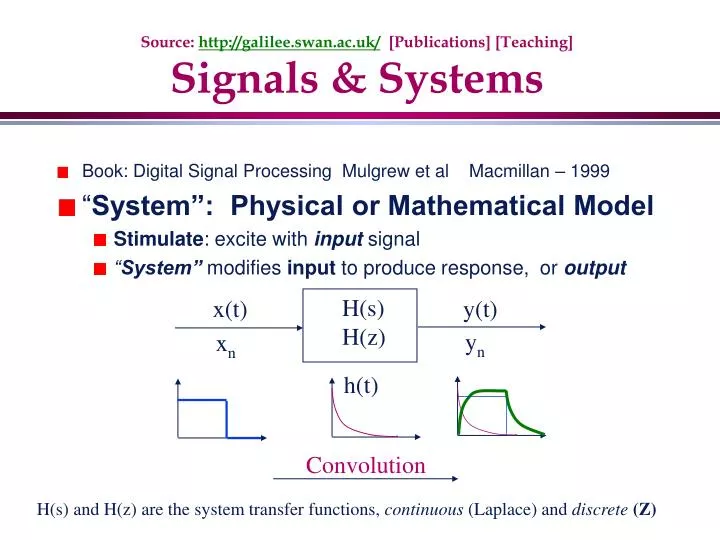
Source: http://galilee.swan.ac.uk/ [Publications] [Teaching] Signals & Systems. Book: Digital Signal Processing Mulgrew et al Macmillan – 1999 “ System”: Physical or Mathematical Model Stimulate : excite with input signal “ System” modifies input to produce response, or output.

E N D
Source: http://galilee.swan.ac.uk/ [Publications] [Teaching]Signals & Systems • Book: Digital Signal Processing Mulgrew et al Macmillan – 1999 • “System”: Physical or Mathematical Model • Stimulate: excite with inputsignal • “System”modifies input to produce response, or output H(s) H(z) x(t) y(t) yn xn h(t) Convolution H(s) and H(z) are the system transfer functions, continuous (Laplace) and discrete (Z)
= H(s) = H(z) H(s) H(z) x(t) y(t) yn xn h(t) Time & Frequency Representations • Fourier Transform: x(t) X() • Laplace Transform: x(t) X(s) • Z Transform: xn X(z) Transfer Functions: Y(s) X(s) Y(z) X(z)
Practical Significance H(s) H(z) x(t) y(t) yn xn h(t) Convolution Replaced by Multiplication Transfer Functions: Y(s) X(s) = H(s) y(t) = L-1{H(s) . X(s)} yn = Z-1{H(z) . X(z)} = H(z) Y(z) X(z) Thus, y(t) or yn can be analytically determined, knowing the transforms of the input and the system transfer function
Jean Baptiste Joseph Fourier Born: 21 March 1768 in Auxerre, Bourgogne Lagrange & Laplace both taught Fourier
Signal Classification • Continuous & Discrete: x(t) & xn • Periodic and Non-Periodic (or Aperiodic) periodic if: x(t) = x(t + T) or xn = xn+N • Energy Signals • Power Signals
Examples • Energy Signals • Power Signals • Consider the case of periodic signals
Fourier Overview • Fourier Series • Fourier Transform • Discrete FT
Fourier Series(1) • Periodic Signals (ie these are “power” signals) can be represented by a weighted sum of sine and cosines:
Fourier Series (2) • In complex form: (k>0)
+V T -V Fourier Series (3) • So, any periodic function, x(t), can be represented by an infinite sum of sine and cosine terms t A0 represents the average (dc) term and by inspection this is zero (prove this by applying equation for Ak )
Fourier Series (4) • To find Ak and Bk : +V t Fix T phase: T -V Now only Bk terms are of interest:
V -V Fourier Series (5)
V -V Fourier Series (6)
V -V Fourier Series (7)
V -V Fourier Series (8) - Odd & Even Here, x(t) is an oddfunction t=0
V -V Fourier Series (9) - Odd & Even Here, x(t) is an evenfunction t=0
Fourier Series (10) cos k0t cos 10t cos 00t 1 sin k0t sin 10t Ak A1 A0/2 Bk B1 x(t)
Fourier Transform Pair • Often derived from the Fourier Series
Fourier Series to Transform (1) V T t
Fourier Series to Transform(2) V T t • Sketch Xk for k = -10,-9,…… 0,1,2, ….. 10 for: • /T = 0.5 • /T = 0.1 • (NB: Xk is a discrete series!)
Fourier Transform Example from Fourier series: V t Fourier transform definition: & 0
Fourier Series Example V T t It can be shown:
Fourier Overview • Fourier Series • Fourier Transform • Discrete FT
Discrete Fourier Transform DFT DFT: IDFT: Differences : 1/N normalizing factor phase: in DFT imaginary terms are -ve. Same algorithm can be used for both DFT and IDFT (with some post-operations)
DFT & IDFT Xk is complex: (R + j I) or { cos( ) + j sin()} xn is very often real - data from the world then k = 0, 1 …. N/2 , since terms for k=N/2-m = terms for N/2+m
Vector/Matrix Interpretation xn Xk = Wkn exp(-j2nk/N
X0 X0 X1 X1 X2 X2 REAL part cos() IMAG. part sin() k Anti-Symmetric about N/2 Symmetric about N/2
X0 X0 X1 X1 X2 X2 ExamplesREAL part cos() IMAG. part sin() xn
Odd and Even Functions(1) Even: f(t)=f(-t) Odd: f(t)=-f(-t)
Odd and Even Functions(2) Even: Odd: Even: Odd:
Odd and Even Functions(3) x(t) = x(-t) Even: x(t) = x(-t) Resultant generally non-zero Symmetry about N/2 in DFT ie do half the work only Even: cos(n) = cos(N-n) f(t) = f(-t)
Odd and Even Functions(4) f(t) = f(-t) Even: f(t) = f(-t) Convolution resultant is always zero Anti-symmetry about N/2 in DFT Odd: sin(n) = -sin(N-n) f(t) = - f(-t)
Fourier/Laplace Transforms Fourier: Laplace: • s = + j Power signals such as unit step Lower limit = 0 for real signals
Fourier/Laplace Transform ofUnit Step Fourier: Laplace: Solution: replace u(t) with exp(- t).u(t) • s = + j Power signals such as unit step Lower limit = 0 for real signals
H(s) H(z) x(t) y(t) yn xn h(t) Convolution H(s) and H(z) are the system transfer functions, continuous (Laplace) and discrete (Z) (Dynamic)Systems • “System”: Physical or Mathematical Model • Stimulate: excite with inputsignal • “System”modifies input to produce response, or output
Transfer Functions, Poles and Zeros (1) • PolesandZerosare roots of atransfer function • drive the function to • Zeros drive the function to zero h(t) x(t) y(t) H(s) Eg: j s = -b Zeros at s=0 & s = -a Poles at s = -b and .. (find the two other x and plot) X 0 -a H(s) and H(z) are the system transfer functions, continuous (Laplace) and discrete (Z)
2 s2 s1 X X 3 j 1 2 s12 X X Transfer Functions, Poles and Zeros (2) • Polesdetermine nature of response, oscillatory or not 1 j j s2 s1 Poles at: X X Key 4 j s2 X 3 s1 X complex roots complexresponse 4
Frequency Response from TF’s (1) j EG1: 1 M (1) X a j EG2: 1 M (1) • Question: • Find phase at 3db • EG1 & EG2
Frequency Response from TF’s (2) EG3: j 1 Mb(1) Ma(1) a b X X j a EG4: 1 Mb(1) Ma (1) b X a
2 s2 s1 X X 3 j 1 2 s12 X X Transfer Functions, Poles and Zeros (3) • Polesdetermine nature of response, oscillatory or not 1 j j s2 s1 Poles at: X X Key 4 j s2 X 3 s1 X complex roots complexresponse 4
2 -b -a X X Transfer Functions, Poles and Zeros (4) • Polesdetermine nature of response, oscillatory or not 1 j j -b -a X X Poles at –a & -b 4 a & b are complex 3 j j b X a=b X X complex roots give complexresponse a X
Transfer Functions, Poles and Zeros (5) 2 • Standard Form: 1 j j Limit before oscillations s2 s1 s1 = s2 X X X X Poles at Complex poles j Limit of stability X s1 & s2 are complex when < 1 3 X Complex pairs complex poles give complex response n X X