Download
1 / 27
270 likes | 593 Views
Simultaneous Localization and Mapping. Presented by Lihan He Apr. 21, 2006. Outline. Introduction SLAM using Kalman filter SLAM using particle filter Particle filter SLAM by particle filter My work : searching problem. Introduction: SLAM. SLAM: Simultaneous Localization and Mapping.

E N D
Simultaneous Localization and Mapping Presented by Lihan He Apr. 21, 2006
Outline • Introduction • SLAM using Kalman filter • SLAM using particle filter • Particle filter • SLAM by particle filter • My work : searching problem
Introduction: SLAM SLAM: Simultaneous Localization and Mapping A robot is exploring an unknown, static environment. • Given: • The robot’s controls • Observations of nearby features The controls and observations are both noisy. • Estimate: • Location of the robot -- localization where I am ? • Detail map of the environment – mapping What does the world look like?
a2 at a1 at-1 … x1 x2 xt xt-1 … x0 o2 o1 ot ot-1 … m Introduction: SLAM Markov assumption State transition: Observation function:
p(xt) p(mt) or mt p(x1) p(m1) or m1 p(xt-1) p(mt-1) or mt-1 … Prior distribution on xt after taking action at Introduction: SLAM Method: Sequentially estimate the probability distribution p(xt) and update the map. Prior: p(x0)
Introduction: SLAM Map representations 1. Landmark-based map representation Track the positions of a fixed number of predetermined sparse landmarks. Observation: estimated distance from each landmark. 2. Grid-based map representation Map is represented by a fine spatial grid, each grid square is either occupied or empty. Observation: estimated distance from an obstacle using a laser range finder.
Represent the distribution of robot location xt(and map mt) by a Normal distribution Introduction: SLAM Methods: The robot’s trajectory estimateis a tracking problem 1. Parametric method – Kalman filter Sequentially update μt and Σt 2. Sample-based method – particle filter Represent the distribution of robot location xt(and map mt)by a large amount of simulated samples. Resample xt (and mt) at each time step
Location error Map error Introduction: SLAM Why is SLAM a hard problem? Robot location and map are both unknown. • The small error will quickly accumulated over time steps. • The errors come from inaccurate measurement of actual robot motion (noisy action) and the distance from obstacle/landmark (noisy observation). When the robot closes a physical loop in the environment, serious misalignment errors could happen.
SLAM: Kalman filter Update equation: Assume: Prior p(x0) is a normal distribution Observation function p(o|x) is a normal distribution Then: Posterior p(x1), …, p(xt) are all normally distributed. Mean μtand covariance matrix Σt can be derived analytically. Sequentially update μt and Σt for each time step t
Assume: State transition Observation function Kalman filter: Propagation (motion model): Update (sensor model): SLAM: Kalman filter
localization mapping SLAM: Kalman filter The hidden state for landmark-based SLAM: Map with N landmarks: (3+2N)-dimentional Gaussian State vector xt can be grown as new landmarks are discovered.
Idea: • Normal distribution assumption in Kalman filter is not necessary • A set of samples approximates the posterior distribution and will be used at next iteration. • Each sample maintains its own map; or all samples maintain a single map. • The map(s) is updated upon observation, assuming that the robot location is given correctly. SLAM: particle filter Update equation:
Particle filter: Assume it is difficult to sample directly from But get samples from another distribution is easy. We sample from , with normalized weight for each xit as The set of (particles) is an approximation of Resamplextfrom ,with replacement, to get a sample set with uniform weights SLAM: particle filter
Particle filter (cont’d): 0.4 0.3 0.2 0.1 SLAM: particle filter
Choose appropriate Transition probability Choose Then Observation function SLAM: particle filter
Algorithm: Let state xt represent the robot’s location, 1. Propagate each state through the state transition probability . This samples a new state given the previous state. 2. Weight each new state according to the observation function 3. Normalize the weights, get . 4. Resampling: sample Ns new states from are the updated robot location from SLAM: particle filter
are the expected robot moving distance (angle) by taking action at. Measured distance (observation) for sensor k Map distance from location xtto the obstacle SLAM: particle filter State transition probability: Observation probability:
SLAM: particle filter • Lots of work on SLAM using particle filter are focused on: • Reducing the cumulative error • Fast SLAM (online) • Way to organize the data structure (saving robot path and map). Maintain single map: cumulative error Multiple maps: memory and computation time • In Parr’s paper: • Use ancestry tree to record particle history • Each particle has its own map (multiple maps) • Use observation tree for each grid square (cell) to record the map corresponding to each particle. • Update ancestry tree and observation tree at each iteration. • Cell occupancy is represented by a probabilistic approach.
Searching problem Assumption: • The agent doesn’t have map, doesn’t know the underlying model, doesn’t know where the target is. • Agent has 2 sensors: • Camera: tell agent “occupied” or “empty” cells in 4 orientations, noisy sensor. • Acoustic sensor: find the orientation of the target, effective only within certain distance. • Noisy observation, noisy action.
Searching problem • Similar to SLAM • To find the target, agent need build map and estimate its location. • Differences from SLAM • Rough map is enough; an accurate map is not necessary. • Objective is to find the target. Robot need to actively select actions to find the target as soon as possible.
Searching problem • Model: • Environment is represented by a rough grid; • Each grid square (state) is either occupied or empty. • The agent moves between the empty grid squares. • Actions: walk to any one of the 4 directions, or “stay”. Could fail in walking with certain probability. • Observations: observe 4 orientations of its neighbor grid squares: “occupied” or “empty”. Could make a wrong observation with certain probability. • State, action and observation are all discrete.
Searching problem In each step, the agent updates its location and map: • Belief state: the agent believes which state it is currently in. It is a distribution over all the states in the current map. • The map: The agent thinks what the environment is . • For each state (grid square), a 2-dimentional Dirichlet distribution is used to represent the probability of “empty” and “occupied”. • The hyperparameters of Dirichlet distribution are updated based on current observation and belief state.
Belief state update: the set of neighbor states of s where Probability of successful moving from sjto s when taking action a From map representation and with Neighbor of s in orientation j Searching problem
Assumeat step t-1, the hyperparameter for state S is At step t, the hyperparameter for state S is updated as and are the posterior after observing o given that the agent is in the neighbor of state s. If the probability of wrong observation for any orientation is p0,then p0 if o is “occupied” 1-p0 if o is “empty” prior can be computed similarly. Searching problem Map update (Dirichlet distribution):
Searching problem Belief state update: a=“up” a=“right” Map representation update: a=“right” a=“up”
Searching problem Choose actions: Each state is assigned a reward R(s) according to following rules: Less explored grids have higher reward. Try to walk to the “empty” grid square. Consider neighbor of s with priority. x x