Download
1 / 136
1.41k likes | 1.66k Views
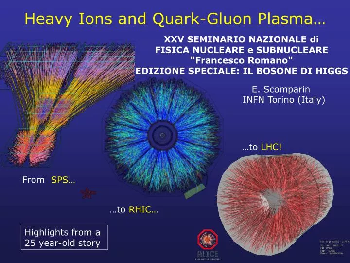
Heavy Ions and Quark-Gluon Plasma…. XXV SEMINARIO NAZIONALE di FISICA NUCLEARE e SUBNUCLEARE "Francesco Romano" EDIZIONE SPECIALE: IL BOSONE DI HIGGS. E. Scomparin INFN Torino (Italy). …to LHC!. From SPS…. …to RHIC…. Highlights from a 25 year-old story . Before starting….

E N D
Heavy Ions and Quark-Gluon Plasma… XXV SEMINARIO NAZIONALE di FISICA NUCLEARE e SUBNUCLEARE "Francesco Romano" EDIZIONE SPECIALE: IL BOSONE DI HIGGS E. Scomparin INFN Torino (Italy) …to LHC! From SPS… …to RHIC… Highlights from a 25 year-old story
Before starting…. • Many thanks to all of my colleagues who produced many of the • plots/slides I will show you in these three lectures….. …and in particular to my Torino colleagues Massimo Masera and Francesco Prino. We hold together a university course on these topics and several slides come from there
Why heavy ions ? • Heavy-ion interactions represent by far the most complex collision • system studied in particle physics labs around the world • So why people are attracted to the study of such a complex system ? • Because they can offer a unique view to understand • The nature of confinement • The Universe a few micro-seconds after the Big-Bang, • when the temperature was ~1012 K • Let’s briefly recall the properties of strong interaction…..
Strong interaction • Stable hadrons, and in particular protons and neutrons, which build up • our world, can be understood as composite objects, made of quarks • and gluons, bound by the strong interaction (colour charge) • 3 colour charge states (R,B,G) are • postulated in order to explain the • composition of baryons (3 quarks or • antiquarks) and mesons (quark-antiquark pair) • as color singlets in SU(3) symmetry • Colour interaction through 8 massless vector • bosons gluons • The theory describing the interactions of quarks and gluons was • formulated in analogy to QED and is called Quantum • Chromodynamics (QCD)
Coupling constant • Contrary to QED, in QCD the coupling constant decreases when • the momentum transferred in the interaction increases or, in other • words, at short distances • Express S as a function of • its value estimated at a certain • momentum transfer • Consequences • asymptotic freedom (i.e. perturbative calculations possible • mainly for hard processes) • interaction grows stronger as distance increases
From a confined world…. • The increase of the interaction strength, when for example a quark and • an antiquark in a heavy meson are pulled apart can be approximately • expressed by the potential where the confinement term Kr parametrizes the effects of confinement • When r increases, the colour field can be seen as a tube connecting the quarks • At large r, it becomes energetically favourable to convert • the (increasing) energy stored in the color tube to a • new qqbar pair • This kind of processes (and in general the phenomenology • of confinement) CANNOT be described by perturbative QCD, but rather through lattice calculations or bag models, inspired to QCD
…to deconfinement • Since the interactions between quarks and gluons become weaker • at small distances, it might be possible, by creating a high • density/temperature extended system composed by a large number of • quarks and gluons, to create a “deconfined” phase of matter • First ideas in that sense date back to the ‘70s ”Experimental hadronic spectrum and quark liberation” Cabibbo and ParisiPhys. Lett. 59B, 67 (1975) Phase transition at large T and/or B
Becoming more quantitative… • MIT bag model: a simple, phenomenological approach which contains • a description of deconfinement • Quarks are considered as massless particles contained in a finite-size bag • Confinement comes from the balancing of the pression from the quark • kinetic energy and an ad-hoc external pressure Kinetic term Bag energy • Bag pressure can be estimated by considering the typical hadron size • If the pression inside the bag increases in such a way that it exceeds the • external pressure deconfined phase, or Quark-Gluon Plasma (QGP) • How to increase pressure ? • Temperature increase increases kinetic energy associated to quarks • Baryon density increase compression
High-temperature QGP • Pressure of an ideal QGP is given by • with gtot(total number of degrees of freedom relative to quark, antiquark • and gluons) given by gtot = gg + 7/8 (gq + gqbar) = 37, since gg = 8 2 (eight gluons with two possible polarizations) gq = gqbar = Ncolor Nspin Nflavour= 3 2 2 • The critical temperature where QGP pressure is equal to the bag • pressure is given by and the corresponding energy density =3P is given by
High-density QGP • Number of quarks with momenta between p and p+dp is (Fermi-Dirac) where q is the chemical potential, related to the energy needed to add one quark to the system • The pressure of a compressed system of quarks is • Imposing also in this case the bag pressure to be equal to the pressure • of the system of quarks, one has • which gives q = 434 MeV • In terms of baryon density this corresponds to nB = 0.72 fm-3, which is • about 5 times larger than the normal nuclear density!
Lattice QCD approach • The approach of the previous slides can be considered useful only • for what concerns the order of magnitude of the estimated parameters • Lattice gauge theory is a non-perturbative QCD approach based on a • discretization of the space-time coordinates (lattice) and on the • evaluation of path integrals, which is able to give more quantitative • results on the occurrence of the phase transition • In the end one evaluates the partition function and consequently • The thermodynamic quantities • The “order parameters” sensitive to the phase transition • This computation technique requires intensive use of computing resources • “Jump” corresponding to the • increase in the number of degrees • of freedom in the QGP • (pion gas, just 3 degrees of freedom, • corresponding to +, -, 0) • Ideal (i.e., non-interacting) gas • limit not reached even at high • temperatures
Phase diagram of strongly interacting matter • The present knowledge of the phase diagram of strongly interacting • matter can be qualitatively summarized by the following plot • How can one “explore” this phase diagram ? • By creating extended systems of quarks and gluons at • high temperature and/or baryon density heavy-ion collisions!
BNL Facilities for HI collisions • The study of the phase transition requires center-of-mass energies of • the collision of several GeV/nucleon • First results date back to the 80’s when existing accelerators and • experiments at BNL and CERN were modified in order to be able to • accelerate ion beams and to detect the particles emitted in the collisions
From fixed-target… • SPS at CERN • p beams up to 450 GeV • O, S, In, Pb up to 200 A GeV • AGS at BNL • p beams up to 33 GeV • Si and Au beams up to 14.6 A GeV Remember Z/A rule !
… to colliders! • RHIC: the first dedicated machine for HI collisions (Au-Au, Cu-Cu) • Maximum sNN = 200 GeV • 2 main experiments : STAR and PHENIX • 2 small(er) experiments: PHOBOS and BRAHMS
… to colliders! • LHC: the most powerful machine for HI collisions • sNN = 2760 GeV(for the moment!) • 3 experiments studying HI collisions: ALICE, ATLAS and CMS
How does a collision look like ? • A very large number of secondary particles is produced • How many ? • Which is their kinematical distribution ?
Kinematical variables • The kinematical distribution of the produced particles are usually • expressed as a function of rapidity (y) and transverse momentum (pT) • pT:Lorentz-invariant with respect to a boost in the beam direction • y: no Lorentz-invariant but additive transformation law y’=y-y • (where y is the rapidity of the ref. system boosted by a velocity ) • y measurement needs particle ID (measure momentum and energy) • Practical alternative: pseudorapidity () y~ for relativistic particles • Alternative variable to pT: transverse mass mT
Typical rapidity distributions Fixed target: SPS • pBEAM=158 GeV/c, bBEAM=0.999982 • pTARGET=0 , bTARGET=0 Midrapidity: largest density of produced particle Collider: RHIC • pBEAM=100 GeV/c • b=0.999956, gBEAM≈100 19
Multiplicity at midrapidity SPS energy RHIC energy LHC energy (ALICE) • Strong increase in the number of produced particles with s • In principle more favourable conditions at large s for the creation of an • extended strongly interacting system
Multiplicity and energy density • Can we estimate the energy density reached in the collision ? • Important quantity: directly related to the possibility of observing • the deconfinement transition (foreseen for 1 GeV/fm3) • If we consider two colliding nuclei with Lorentz-factor , in the instant • of total superposition one could have at RHIC energies (enormous!) • But the moment of total overlap is very short! • Need a more realistic approach • Consider colliding nuclei as thin pancakes (Lorentz-contraction) • which, after crossing, leave an initial volume with a limited longitudinal • extension, where the secondary particles are produced
Multiplicity and energy density • Calculate energy density at the time f (formation time) when the • secondary particles are produced • Let’s consider a slice of thickness z and transverse area A. It will • contain all particles with a velocity (y~ when y is small) The number of particles will be given by
Multiplicity and energy density • The average energy of these particles is close to their average • transverse mass since E=mTcosh y ~ mT when y0 • Therefore the energy density at formation time can be obtained as Bjorken formula • Assuming f ~ 1 fm/c one gets • values larger than 1 GeV/fm3! • Compatible with phase transition • With LHC data one gets Bj ~ 15 GeV/fm3 • Warning: f is expected to decrease when increasing s • For example, at RHIC energies a more realistic value is f~0.35-0.5 fm/c
Time evolution of energy density • One should take into account that the system created in heavy-ion • collisions undergoes a fast evolution • This is a more realistic evaluation (RHIC energies) Peak energy density Energy density at thermalization Late evolution: model dependent
Time evolution of the collision • More in general, the space-time evolution of the collision is not trivial • In particular we will see that different observables can give us • information on different stages in the history of the collision • Soft processes: • High cross section • Decouple late indirect signals for QGP EM probes (real and virtual photons): insensitive to the hadronization phase • Hard processes: • Low cross section • Probe the whole evolution of the collision
High- vs low-energy collisions • Clearly, high-energy collisions should create more favourable • conditions for the observation of the deconfinement transition • However, moderate-energy collisions have interesting features • Let’s compare the net baryon rapidity distributions at various s • Starting at top SPS energy, we observe • a depletion in the rapidity distribution • of baryons (B-Bbar compensates for • baryon-antibaryon production) • Corresponds to two different regimes: • baryon stopping at low s • nuclear transparency at high s Explore different regions of the phase diagram
Mapping the phase diagram High-energy experiments Low-energy experiments • High-energy experiments create conditions similar to Early Universe • Low-energy experiments create dense baryonic system
Characterizing heavy-ion collisions • The experimental characterization of the collisions is an essential • prerequisite for any detailed study • In particular, the centrality of the collision is one of the most important • parameters, and it can be quantified by the impact parameter (b) • Small b central collisions • Many nucleons involved • Many nucleon-nucleon collisions • Large interaction volume • Many produced particles • Large b peripheral collisions • Few nucleons involved • Few nucleon-nucleon collisions • Small interaction volume • Few produced particles 28
Hadronic cross section • Hadronicpp cross section grows logarithmically with s Mean free path LHC(p) RHIC (top) LHC(Pb) SPS • ~ 0.17 fm-3 • ~70 mb • = 7 fm2 ~ 1 fm • is small with • respect to • the nucleus size • opacity Laboratory beam momentum (GeV/c) • Nucleus-nucleus hadronic cross section can be approximated • by the geometric cross section hadPbPb = 640 fm2 = 6.4 barn (r0 = 1.35 fm, = 1.1 fm)
Glauber model • Geometrical features of the collision determines its global characteristics • Usually calculated using the Glauber model, a semiclassical approach • Nucleus-nucleus interaction incoherent superposition of • nucleon-nucleon collisions calculated in a probabilistic approach • Quantities that can be calculated • Interaction probability • Number of elementary nucleon-nucleon • collisions (Ncoll) • Number of participant nucleons (Npart) • Number of spectator nucleons • Size of the overlap region • …. • Nucleons in nuclei considered as point-like and non-interacting • (good approx, already at SPS energy =h/2p ~10-3 fm) • Nucleus (and nucleons) have straight-line trajectories (no deflection) • Physical inputs • Nucleon-nucleon inelastic cross section (see previous slide) • Nuclear density distribution
Nuclear densities Core density “skin depth” Nuclear radius
Interaction probability and hadronic cross sections • Glauber model results confirm the “opacity” of the interacting nuclei, • over a large range of input nucleon-nucleon cross sections • Only for very peripheral collisions (corona-corona) some transparency • can be seen
Nucleon-nucleon collisions vs b • Although the interaction probability practically does not depend on • the nucleon-nucleon cross section, the total number of nucleon-nucleon • collisions does inel corresponding to the main ion-ion facilities
Number of participants vs b • With respect to Ncoll, the dependence on the nucleon-nucleon cross • section is much weaker • When inel > 30 mb, practically all the nucleons in the overlap region • have at least one interaction and therefore participate in the collisions inel corresponding to the main ion-ion facilities 34
Centrality – how to access experimentally • Two main strategies to evaluate the impact parameter in • heavy-ion collisions • Measure observables related to the energy deposited in the • interaction region charged particle multiplicity, transverse • energy ( Npart) • Measure energy of hadrons emitted in the beam direction • zero degree energy ( Nspect)
…and now to some results… • Can we understand quantitatively the evolution of the fireball ?
Chemical composition ofthe fireball • It is extremely interesting to measure the multiplicity of the various • particles produced in the collision chemical composition • The chemical composition of the fireball is sensitive to • Degree of equilibrium of the fireball at (chemical) freeze-out • Temperature Tchat chemical freeze-out • Baryonic content of the fireball • This information is obtained through the use of statistical models • Thermal and chemical equilibrium at chemical freeze-out assumed • Write partition function and use statistical mechanics • (grand-canonical ensemble) assume hadron production is a • statistical process • System described as an ideal gas of hadrons and resonances • Follows original ideas by Fermi (1950s) and Hagedorn (1960s)
Hadron multiplicities vss • Baryons from colliding • nuclei dominate at low s • (stopping vs transparency) • Pions are the most • abundant mesons (low • mass and production • threshold) • Isospin effects at low s • pbar/p tends to 1 at • high s • K+ and more produced • than their anti-particles • (light quarks present in • colliding nuclei)
Statistical models • In statistical models of hadronization • Hadron and resonance gas with baryons and mesons • having m 2 GeV/c2 • Well known hadronic spectrum • Well known decay chains • These models have in principle 5 free parameters: • T : temperature • mB : baryochemical potential • mS : strangeness chemical potential • mI3 : isospin chemical potential • V : fireball volume • But three relations based on the knowledge of the initial state • (NS neutrons and ZS “stopped” protons) allow us to reduce the • number of free parameters to 2 Only 2 free parameters remain: T and mB
Particle ratios at AGS • Results on ratios: cancel a significant fraction of systematic uncertainties • AuAu - Ebeam=10.7 GeV/nucleon - s=4.85 GeV • Minimum c2 for: T=124±3 MeV mB=537±10 MeV c2 contour lines
Particle ratios at SPS • PbPb - Ebeam=40 GeV/ nucleon - s=8.77 GeV • Minimum c2 for: T=156±3 MeV mB=403±18 MeV c2 contour lines
Particle ratios at RHIC • AuAu - s=130 GeV • Valore minimo di c2 per: T=166±5 MeV mB=38±11 MeV c2 contour lines
Thermal model parameters vs. s • The temperature Tch quickly • increases with s up to ~170 MeV • (close to critical temperature for the • phase transition!) at s ~ 7-8 GeV • and then stays constant • The chemical potential B decreases • with s in all the energy range • explored from AGS to RHIC
Chemical freeze-out and phase diagram • Compare the evolution vss of the (T,B) pairs with the QCD phase • diagram • The points approach the phase transition region already at SPS energy • The hadronic system reaches chemical equilibrium immediately after • the transition QGPhadronstakes place
News from LHC • Thermal model fits for yields • and particle ratios • T=164 MeV, excluding protons • Unexpected results for protons: abundances below thermal model • predictions work in progress to understand this new feature!
Chemical freeze-out • Fits to particle abundances • or particle ratios in • thermal models • These models assume • chemical and thermal • equilibrium and describe • very well the data • The chemical freeze-out • temperature saturates • at around 170 MeV, while • B approaches zero at • high energy • New LHC data still • challenging
Collective motion in heavy-ion collisions (FLOW) Radial flow connection with thermal freeze-out Elliptic flow connection with thermalization of the system Let’s start from pT distributions in pp and AA collisions
pTdistributions • Transverse momentum distributions of produced particles can provide important information on the system created in the collisions • Low pT(<~1 GeV/c) • Soft production • mechanisms • 1/pTdN/dpT ~exponential, • Boltzmann-like and almost • independent on s • High pT (>>1 GeV/c) • Hard production • mechanisms • Deviation from exponential • behaviour towards • power-law
Let’s concentrate on low pT • In pp collisions at low pT • Exponential behaviour, identical for • all hadrons (mTscaling) • Tslope~ 167 MeV for all particles • These distribution look like thermal spectra and Tslope can be seen as • the temperature corresponding to the emission of the particles, when • interactions between particles stop (freeze-out temperature, Tfo) 49
pTand mTspectra • Slightly different shape of spectra, • when plotted as a function of pTor mT Evolution of pT spectra vsTslope, higher T implies “flatter” spectra