Download

1 / 26
260 likes | 402 Views
Geolocation of Icelandic Cod using a modified Particle Filter Method. David Brickman Vilhjamur Thorsteinsson. What does one do when …. The best that a “standard” particle filter can do is. model recap position. 600m. 200m. DST recap position.

E N D
Geolocation of Icelandic Cod using a modified Particle Filter Method David Brickman Vilhjamur Thorsteinsson
The best that a “standard” particle filter can do is model recap position 600m 200m DST recap position • Note that the T simulation is good, but the recapture estimate is way off • Note that track goes into deep water – not considered likely for Icelandic Cod • Varying parameters improves results but not by that much. DST tag position model simulation
Why does this occur?? • T field around Iceland is ~ parabolic so that particles drifting from tag location, and trying to follow T data, have 2 possible directions to choose. Climatological September T at 100m Temperature field ~ parabolic • Aside: T field for this study comes from a state-of-the-art circulation model for the Iceland region developed by Kai Logemann (Logemann and Harms Ocean Sci., 2, 291–304, 2006)
OPTIONS • Accept that this is the best that the PF method can do and • Do nothing • Hide these results (~5 out of 27) • See whether modifications to the PF method can produce better simulations
The Data: 27 useable DSTs Example of tag being inserted into cod fish (from Star-Oddi website)
xn+1 dx Vdt xn “Standard” Particle Filter (PF-1) (Andersen et al. 2007, CJFAS 64:618-627) Particles start at the initial tagging position, and evolve according to a Movement model: • Where • xn = (lon,lat) position at time n = the “state” • V = (max) swim velocity = model parameter • U = random # from uniform distribution • dx = change in (lon,lat) position • dt = timestep • particle z-level = DST z-level
Observation model: • Where • yn = observation at time n (i.e. temperature) from the DST • NB: last time includes the “recapture” observation • e = error • g(x) is the model temperature field at x derived from a numerical circulation model
Error Model -- Particle Filter Weight: • Standard assumptions for a SIR filter yield: • The probability of the observation given the state is • and following Andersen et al. (and others):
Particle Filter: “PF-1” • At t=0 NP particles are seeded at the (known) DST tagging position • Each particle evolves according to the movement model • (A) At each timestep evaluate P particle filter weights w • (B) Sample with replacement NP particles from w, preferentially choosing those with higher probability (i.e lower error). Use the standard SIR cumulative distribution method. • (C) Propagate these particles to the next step • Repeat A-C • Continue to end of series, at which time the recapture position is an (important) observation to be incorporated into P. • NB: no backward smoothing procedure coded.
Example of a Good Result Standard PF PF-1 However, note that offshelf drift is not considered biologically realistic
Modifications to standard PF • Two modifications added: • “Attractor” function:To increase the influence of the final (recapture -- R) position, a time-dependent term was added to the error model: distance from recapture position factor that increases as final time is approached • Allows a future observation to influence present state • Adds 2 parameters: time0 and ta
recap position 1 2 Interpretation of Attractor term • Consider 2 particles returning the same T (i.e. T-error) – late in the simulation • The estimate reported by particle 2 is considered more likely because it is closer to the recapture position.
Demersal error term: • Intended to correct the tendancy for particles to follow increasing temperatures by drifting southward • Observed in many simulations but considered biophysically unlikely. • where zni is the depth of the i-th particle at time n (= DST depth) and zbtm(xni) is the model bottom depth at location xni • td is a vertical scale parameter
1 2 Interpretation of Demersal term • Assumes that the school of fish are clustered within td of the bottom and penalizes those fish that do not fit into this “demersal” vertical distribution. • Consider 2 particles at the same depth, reporting the same T • the estimate reported by particle 2 considered more likely as that fish is exhibiting a more demersal behavior. • Action ~ negative diffusion
New Error Model • New terms incorporated in an error distribution (at every timestep, for each particle): • E = S {T-error + attractor-term + demersal-term} • i.e. additive error distribution of un-normalized error terms, sampled using a SIR-type procedure; Preferentially choose particles with lowest error
How to think about this -- Heuristically • For this type of problem (i.e. DST) the backward smoothing procedure is essential as it is the way that the recapture observation influences the solution: • Up to recap obs, PF yields optimal “local” solution • Use of backward smoothing produces optimal “global” solution. • E-distribution “attempts” to solve the global problem in one pass through the data.
Regarding E -- Consider minimizing a likelihood function over all observations: • BTW: solved L(y|q) for optimal parameters using a Direct Search algorithm. • DS algorithm: see Kolda et al. 2003, SIAM V.46, no.3, pp.385-482
shallow shallow xn+1 dx Vdt xn deep deep Note that the Demersal term could be incorporated into the Movement Model by including bathymetry: Present model Model using bathymetry xn+1 Vdt dx xn
Addition of Attractor function only (PF-2) Cf: no attractor
Addition of Attractor function plus Demersal term (PF-4) Cf: attractor only
Summary / Conclusion • Standard PF seen to perform poorly on a number of DSTs • PF method modified by adding: • Attractor term that “sucked” particles toward the recapture position • allows future data to influence present result • Demersal term that favoured particles that adhered to a “gadoid-type” behavior • keeps particles onshelf • Attractor + demersal terms can be considered to be rules or behaviors imposed on the particles. • Result likely depends on Temperature field: • demersal term may not be necessary
Modified PFs performed better than standard PF, especially on difficult DSTs. • However, • Forcing better biological behavior (addition of demersal term) resulted in poorer simulation of temperature timeseries. • i.e. quantitatively WORSE results “Best” result is subjective OR When signal processing theory meets fisheries biology adjustments may have to be made