Download
1 / 26
260 likes | 373 Views
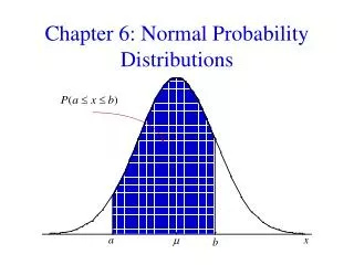
Normal Probability Distributions. Review relative frequency histogram. Values of a variable, say test scores. 1/10 2/10 4/10 2/10 1/10. 60 70 80 90. In this example 10 people took a test. The height of each

E N D
Review relative frequency histogram Values of a variable, say test scores 1/10 2/10 4/10 2/10 1/10 60 70 80 90 In this example 10 people took a test. The height of each bar is the relative frequency or percentage of those in that range of scores. What % of people had test scores between 70 and 80? 40% What % of people had scores less than 70? 30% If you add up all the fractions what do you get? 1
My example on the previous slide is about test scores. Test score is a quantitative variable and the authors suggest that to describe the distribution 1) Plot the data and/or make some sort of graph, 2) Look for the overall pattern – shape, center, and spread, and 3) Calculate a measure of center and spread. The authors suggest that the overall pattern of a large number of observations can be described by a smooth curve called a density curve. A density curve is a mathematical model for a distribution. We use the density curve when we have a real world data pattern that is reasonably enough like the model.
A density curve has the following properties: 1) Is always on or above the horizontal axis, and 2) Has area exactly 1 underneath it. A density curve describes the overall pattern of a distribution. The area under the curve and above any range of values is the proportion of all observations that fall in that range. Back on slide 2 here we do not have a density curve because it is not smooth. But if we smoothed it out it would have the properties we have here. Imagining what we have on slide 2 is smooth, what proportion of values are between 60 and 90? The answer is .8. Note that here that would mean 8 of the 10 people who took the test had a score between 60 and 90.
The Normal Distributions - Basic idea • The normal distribution is a tool we use to try to convey the same information as we get from a relative frequency histogram. • The normal distribution has been used a lot in statistics and we will use it later, so we will look at some details about it. • But, first let’s look at circles - yes I mean circles!
circles and density • Imagine you are at the intersection by Dairy Queen. Now imagine a large circle is placed on the earth such that the center of the circle is at the intersection plus enough houses have been included so 1,000,000 people live in the circle. • New York City has a similar intersection and circle, except the circle is smaller (WHY?).
circles and density • The New York circle is smaller because you travel a shorter distance from the center to get an equal density of people in New York. • The smaller circle in a sense has a smaller standard deviation(actually it has a smaller radius) - the distance is less spread out. • One thing similar about the two circles is that you can divide them both up into quarters. Let’s do this on the next screen with two circles
circles and density A a 25% of the area is in A on the large circle and 25% of the area of the small circle is in part a. How can they both be 25%? It is 25 % of its own total. There are as many different normal distributions as there are circles. BUT, normal distributions are divided up, not into quarters, but in another way.
The Normal Distributions - normal dist. and density • Normal distributions can roughly be drawn by modifying a circle. flip this part out to left flip this part out to right like this
The Normal Distributions - normal dist. and density • Let’s label parts of the normal distributions. This point on the number line is directly below the inflection point. It turns out that the point on the number line is one standard deviation away from the center. This point is where the bottom part of the circle flipped. Let’s call it the inflection point. There is one on the other side as well. number line for the variable- like test score This is the center of the distribution. It really is the mean value.
On the previous screen we see a graph of a normal distribution. Let’s consider an example to highlight some points. Say a company has developed a new tire for cars. In testing the tire it has been determined that the mean tire mileage is 36,500 miles and the standard deviation is 5000 miles. Along the horizontal axis we measure tire mileage. The normal distribution rises above the axis. Note the highest point of the curve occurs above the mean - in our tire example we would be at 36,500. On the curve we have two inflection points, and these occur 1 standard deviation away from the mean. So, mileages 31,500 and 41,500 are 1 standard deviation for the mean and the inflection points occur above them.
The Normal Distributions - notation • In general, now, we will talk about a variable having a normal distribution. We will say variable X is normally distributed with mean mu and standard deviation sigma. • More simply, we say X is N(mu,sigma). • Don’t let the N(---) part fool you, it means N(mean value listed first, then standard deviation value listed).
The Normal Distributions - example with graphical thinking • Say we have a variable X is N(3, 1) Why is this dot, and the one across, above #’s 2 and 4? X is measured on the line 4 2 3 Use the dots as your guide to draw the normal dist. 3 is the mean
The Normal Distributions - another example with graphical thinking • Say we have a variable X is N(3, 2) Why is this dot, and the one across, above #’s 1 and 5? X is measured on the line 4 5 1 2 3 Use the dots as your guide to draw the normal dist. 3 is the mean
The Normal Distributions - compare the two examples • here is what the two examples look like, one on top of the other X is N(3, 1) X is N(3, 2) 4 5 1 2 3
The Normal Distributions - compare the two examples • Note on the previous screen how the X is N(3, 2) had its inflection points wider than on the X is N(3, 1). • Remember how we labeled the quarters of the different circles A and a. We said there was 25% of the circle in both A and a, but based on its own total. • Normal dist.’s have a similar rule. 68% of the area under the curve is between the two inflection points. There is more.
The Normal Distributions - 68-95-99.7 rule • On any normal distribution the inflection points will be 1 standard deviation on either side of the mean. 68% of the area under the curve will be within this one standard dev. • By moving out 2 standard deviations on either side of the mean you have about 95% of the area under the curve. • By moving out 3 stand. dev.’s you have 99.7 % of the area under the curve.
The Normal Distributions - 68-95-99.7 rule • What is the meaning of the phrase, “1 standard dev. on either side of the mean?” • The answer may best seen by an example. X is (10, 2.5) means X is normal with mean 10 and standard deviation 2.5. Thus 7.5 is 1 stand. dev. on the low side of the mean and 12.5 is 1 stand. dev. on the high side of the mean. Thus being anywhere from 7.5 to 12.5 is within 1 standard deviation of the mean.
Note about normal distribution: 1. There are many normal distributions, each characterized by a mean value and a standard deviation. 2. The high point of the curve is above the mean and for a normal distribution the mean = median = mode. 3. Depending on the variable, the mean can be negative, zero, or positive. 4. The normal curve is symmetric. This means each side is a mirror image of itself. 5. Larger standard deviations result in a flatter, wider distribution. 6. Probabilities for the variable are found from areas under the curve - the 68, 95, 99.7 rule is an example of this.
26,500 31,500 36,500 41,500 46,500 miles -2 -1 0 1 2 z Note the concept of a z score for a value for a variable. Using the tire example from a few slides back: z = ( a value minus the mean)/standard deviation. So the value 26,500 has a z = (26,500 - 36,500)/5000 = -2. This means 26,500 is 2 standard deviations below the mean. You can check the other values.
So, from the previous slide we see that approximately 68% of all the tires will last between 31,500 and 41,500 miles. Approximately 95% of the tires will last between 26,500 and 46,500 miles. Approximately 99.7% of the tires will last between 21,500 and 51,500 miles. This approximation rule is useful to make a quick set of calculations that are roughly correct about a distribution that is normal. Sometimes we want to make more accurate statements about a normal distribution. We turn to that next.
The standard normal distribution Remember how we said there are many different circles and many different normal distribution? Sure you do. The z value translates any normally distributed variable into what is called the standard normal variable. Technically the picture I have on the previous screen is misleading because the z’s are a different scale than the miles, but don’t worry. In the book there is a table with z values and areas under the curve. Let’s see how to use the table. Here is one place where I want you to be extra careful when you calculate z. Round z to 2 decimal places. In general the z value can be thought of as a.bc. To use the table we break up a.bc into a.b and .0c For example the number 2.13 is broken up into 2.1 and .03
Using the standard normal table The z = 2.13 means we should go down the table to 2.1 and then over to .03. The number in the table is .9834. This means the probability of getting a value less than z = 2.13 is .9834. In the tire example if we look at the mean value 36,500, we see the z = (36,500 - 36,500)/5000 = 0.00 and in the table we see the value .5000. Thus, there is a .5 probability the tire mileage will be less than 36,500. So the table has the area under the curve to the left of the value of interest. We may want other z’s and other areas. What do we do?
Say we want the area to the right of a z that is greater than 0? The table has the area to the left. Whatever the z is, go into the table and get the area and then take 1 minus the area in the table. The z here would be negative. Say we want area b. Area a is in the table and b is 1 minus area a. b a Area b would be found in a similar way to what is above.
Back in the old days when I had to walk to school uphill both ways in three feet of snow, the standard normal table was all we had to calculate probabilities for a normal distribution. Now we have Microsoft Excel to make the calculations. This is not a class in Excel – but I show you if you like Excel. The NORMSDIST function assumes we have a z value and we want to find the area to the left of the z - the area to the left is the cumulative probability. The function has the form =NORMSDIST(z), where z is the value we have. z can be negative in Excel. The NORMDIST function allows us to just work with the variable without getting the z and we can still have the cumulative probability. The function has the form =NORMDIST(value, mean, standard deviation, TRUE). This is an innovation of Excel over the old days.
Sometimes we may have an area and want to know the z. The function NORMSINV asks us to give an area to the left of a value and the function will give us the z value. The form of the function is =NORMSINV(cumulative probability). The function NORMINV does the same, except not in z value form. It just give the value in the same form as the variable. The form of the function is =NORMINV(cumulative prob, mean, standard deviation)