Download
1 / 62
630 likes | 776 Views
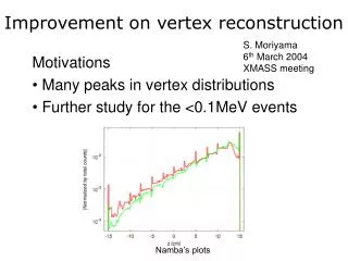
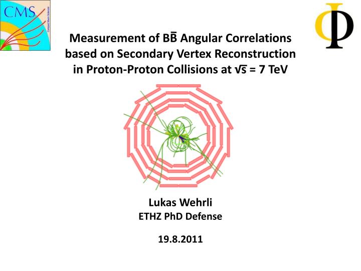
Measurement of BB Angular Correlations based on Secondary Vertex Reconstruction in Proton-Proton Collisions at √s = 7 TeV. Lukas Wehrli ETHZ PhD Defense 19.8.2011. Outline. Introduction to Beauty Physics and Motivation The LHC and the CMS experiment B-tagging and Vertex Reconstruction

E N D
Measurement of BB Angular Correlations based on Secondary Vertex Reconstruction in Proton-Proton Collisions at √s = 7 TeV Lukas Wehrli ETHZ PhD Defense 19.8.2011
Outline • Introduction to Beauty Physics and Motivation • The LHC and the CMS experiment • B-tagging and Vertex Reconstruction • Inclusive Vertex Finder • B anti-B Correlation Analysis • Systematic Uncertainties • Results • Conclusion and Outlook 1
Standard Model of Particle Physics u c t Quarks Strong: gluons s d b Charged Leptons • Standard Model: elementary particles (quarks, leptons) and fundamental interactions (weak, electromagnetic, strong) • Quantum Chromodynamics: Quantum field theory of strong interaction. Confinement: free quarks not observed, quarks form hadrons. • Beauty physics: b quarks or hadrons containing b quarks involved. Electromagnetic: g m e t Weak: W+, W-, Z0 Neutral Leptons ne nt nm u c t Quarks Strong: gluons s d b Charged Leptons Electromagnetic: g m e t Weak: W+, W-, Z0 Neutral Leptons ne nt nm 2
Beauty Physics at LHC • Large bb cross section • (b produced in pairs through strong interaction) • studies with early data possible. • b quarks are a key ingredient at LHC • as signal (top, low mass Higgs, new physics). • as background to new physics searches. • Measure • b production (cross section). • bb pair dynamics. 3
Proton-Proton Scattering b-jet B b Measured in detector b-jet b B Hard Scattering Protons Hadronization Bunches of particles: Jets 4
Angular Correlations BB production can be divided into three mechanisms: • Flavor Creation (FCR) • Flavor excitation (FEX) • Gluon splitting (GSP) Angular correlations allow to study different productions: FCR:Momentum conservation requires b/b to be back-to-back in azimuthal angle. GSP: b/b produced with small opening angle. • Need to find B hadrons with good angular resolution LO NLO GSP FCR • BB production and angular correlation study: • Dynamics of hard scattering process within pQCD. • Test of pQCD LO and NLO cross sections. • Hadronization properties of heavy quarks. DR between B hadrons 5
Large Hadron Collider CMS LHC (27km) LHCb ALICE SPS (7km) ATLAS • Proton-proton collisions since 2009 • 27 km long ring tunnel (from LEP) • 4 experiments • Nov. 23, 2009: • first collisions at 900 GeV • Since March 30, 2010: • collisions at 7 TeV • Integrated Luminosity (CMS): 2.4 fb-1 6
Compact Muon Solenoid Diameter: 15 m Length: 21.6 m Weight: 12000 t Magnet: 3.8 T Tracking: Silicon Strips and Pixels Calorimeter: ECAL: PbWO4 crystals + preshower HCAL: Brass absorber and scintillators Steel return yoke (2T) instrumented with Muon spectrometer: Drift Tube Chambers, Cathode Strip Chambers, Resistive Plate Chambers Data reduction (not all collision events stored): Trigger: Level 1: 40‘000 kHz 100 kHz High-Level-Trigger: 100 kHz 100 Hz 7
B Correlation Analysis Goal: MeasureDfbetweentwo B hadrons. (or , angle in 3D). p p collision B hadrons Other (D) hadrons r, f: cylindrical coordinates q: polar angle h: pseudorapidity f r q z Df B hadrons are long living particles (ct about 500mm)… 8
B Correlation Analysis B hadrons??? B jets??? 9
B-tagging 0.67 0.78 Jets 0.22 0.16 • Identify jets originating from b quarks. • Associate real number, a “discriminator”d to each jet. • Different algorithms exploit long life time of B, semi-leptonic decay mode, high B mass,… • Input: Jets, Tracks, Primary Vertex, Leptons. • For first data: Simple Secondary Vertex (SSV) Track Counting (TC) • SSV: Reconstructs the B decay vertex using an adaptive vertex fitter. Vertex decay length significance sSV used for d. b-tagging Discriminators dsv SV PV 10
B Correlation Analysis -1 B hadrons -1 -1 -1 -1 -1 -1: no vertex reconstructed >2: likely a B jet Df 2.51 3.04 11
Small Opening Angles 2 B in one Jet • For small opening angle between B in pair: both B merged into one single jet. • GSP contribution expected to be large. • Measure angle between B flight directions (not jets). Flight direction: Vector from primary to secondary Vertex. large opening angle small SV SV SV SV PV PV 12
B Correlation Analysis Primary Vertex Secondary Vertices (from B hadron decays) 13
B Correlation Analysis Primary Vertex Angle Secondary Vertices (from B hadron decays) 13
Vertex Reconstruction Two steps: - Vertex finding(cluster tracks with common origin) - Vertex fitting(computation of best vertex parameters). Adaptive Vertex Reconstructor (AVR): • Use all tracks for finding PV. • One cluster of tracks per jet (DR < 0.3 between track and jet axis). Adaptive Vertex Fitter (AVF): • Iterative re-weighted Kalman Filter. • Outlying tracks down-weighted. AVR AVF 14
Jets with Two B Standard Vertex Finder (AVR): • Clusters tracks in cone around jet axis (DR = 0.3). • Secondary vertices reconstructed with high efficiency. Jets containing two B hadrons: • AVF used iteratively, reconstruction of several vertices per cluster possible. • But: jet direction is no good estimate for B flight direction. Need vertex finder independent of any jet direction: „Inclusive Vertex Finder“. standard track acceptance cone 15
Inclusive Vertex Finder • Inclusive Vertex Finder (IVF) does not use jet directions as input, designed to be able to reconstruct both B also for small bb separation angle. • Algorithm: Seeds: start with good tracks with high impact parameter and impact parameter significance. Cluster tracks compatible to make a vertex with the seed track. Use AVF and AVR for vertex fitting. Clean up duplicates. • IVF can be used also in other analyses (e.g. Higgsbb). PV 1. Seed tracks with high IP significance 3. Fit Secondary Vertices using the AVF and AVR 2. Cluster tracks compatible with seed 16
Analysis Overview Trigger & event selection • Single jet trigger above 15, 30 and 50 GeV. • Hardest anti-ktjet: |h|<3.0, corrected pTsuch thatHLT efficiency > 99%: 56, 84, 120 GeV. Analysis strategy • Apply cuts to select B vertices. • Combine vertices from BDX decays into a single B candidate. • Select events with exactly two B candidates (scalar mass sum > 4.5 GeV). • 160, 380 and 1038 events in total for three leading jet pTregions p B D B B COMBINE KEEP PV PV 17
Resolution and Efficiency SV B B DRvv Leading jet pT > 84 GeV DRBB SV • DRVV versus DRBB(left) DRVV - DRBB and (right) • Below 4 % of events out of diagonal (|DRVV-DRBB | > 0.2) • DR resolution (0.02) much smaller than bin width (0.4). • Calculate efficiency and purity on MC as function of • leading jet pT and DR and apply correction bin-wise. 18
Measured B Candidate Properties Leading jet pT > 84 GeV • Vertex mass (left) and 3D flight distance significance (right) • All selection cuts applied (apart from those on shown quantities) • Simulation normalized to number of data events • Very nice agreement between MC and data • Small excess in data mass distribution at 1.7 GeV (16 %) • larger charm contribution in data? 19
Systematic Uncertainties • Uncertainties on the shapeand on the absolutenormalization treated separately. • Normalization uncertainties large (43 %). Dominant contribution: uncertainty on efficiency of B hadron reconstruction (20 % for one vertex, estimated from standard b-tagging efficiency studies 40 % for two vertices). • Shape uncertainties around 16 %. Dominant contributions from MC statis-tical uncertainty (13 %) and uncertainty on phase space correction (8 %). • Statistical and systematic uncertainties added in quadrature. • Possible way to reduce normalization uncertainties: Comparison of SV based analysis to jet based analysis for well separated B hadrons (DR > 1.0). 20
Algorithmic Effects (Data Mixing) At small DR an algorithmic efficiency loss is expected for B hadron reconstruction • MC description of algorithmic efficiency verified with a data mixing technique: • Select events with one reconstructed B candidate • Mix pairs of events if PV positions compatible (20 mm) • Mixed event re-reconstructed (tracking, vertex finding and fitting rerun) • Compare relative efficiency of reconstructing both B candidates in data and simulation (shape) • Systematic uncertainty estimated to be 2 %. 21
Results • Differential cross section distributions in DR and Df: • Total measured cross sections: • for leading jet pT > 56, 84 and 120 GeV. measured events in bin bin purity total bin efficiency bin width, A is DR or Df integrated luminosity Visible phase space: |h|<3.0 for leading jet, pT(B) > 15 GeV, |h(B)| < 2.0 22
Results • Ratio:sDR<0.8/sDR>2.4 (GSP/FCR region) • Relative amount of GSP with respect to FCR for different event energy scales. • Symbols plotted at the mean leading jet pT of the bin. • GSPsignificantly exceeds FCR. • Relative amount of FCR and GSP changes with event energy scale. • General trend described by MC. • Pythia: overestimation of back-to-back contribution. MadGraph: overestimation of collinear contribution. JHEP 1103 (2011) 136 23
Differential Cross Section • Data and Pythia compared for three leading jet pTregions • Simulation: relative normalization (see below) • pT> 56 and pT> 84 GeV bins offset by factor 4 and 2 • Uncertainty due to absolute normalization (43%) not included • Normalization to FCR region: normalize to cross section in DR > 2.4 (Df>3p/4) • (back-to-back topology, LO dominated). • Systematic uncertainties on absolute normalization irrelevant. 24
Comparison to Theoretical Predictions • Data and different predictions (MC@NLO, MadGraph, Cascade) normalized to Pythia prediction. • Relative normalization • (DR>2.4, Df>3p/4, shaded) • No model matches data very well • Data in between Pythia and MadGraph for small angles • Cascade and MC@NLO under-estimate contribution at small DR • MC@NLO prediction for Df pretty accurate (not shown) 25
Conclusion and Outlook • First measurement of B anti-B angular correlations at 7 TeV. • Measure correlations using secondary vertices in full angular range, accessing collinear region. • Novel vertex finding technique independent of jet reconstruction developed. The Inclusive Vertex Finder is well suited for any kind of study using secondary vertices. • Collinear B production is a sizable fraction of the total cross section. The relative amount is increasing with the event energy scale. • General prescription of pQCD confirmed. None of the LO or NLO predictions describes the data very well. Input for theory and MC event generators. 26
Special thanks to… …everybody who contributed to this work. • My supervisors • People in our group at the IPP • People from University of Zurich • People from the CMS collaboration • CERN staff • Many more… 27
MC Event Generation MC Event Generation • Hard event scattering (black) • Initial state parton shower (blue) • Final state parton shower (green) • Parton density functions (red) • Cluster/String formation (purple) • Hadron decay (brown)
MC Event Generators MC event generator settings: Pythia: all-order multipurpose programm. ME at LO, PS for more activity MC@NLO: NLO QCD massive matrix element calculations matched with PS (Herwig). MadGraph: Hybrid solution between 22 and NLO simulations, matching scheme to avoid double counting (PS). Cascade: based on LO ME using high-energy factorization, convoluted with unintegrated parton distributions.
CMS Silicon Pixel Detector • Silicon pixel detector (66 Mio. pixels, size: 100x150mm ATLAS: 50x400mm). • Three barrel layers, two endcap disks covering |h|<2.5. • 100 million particles per cm2 and s at full luminosity. • Analog readout (charge sharing better spatial resolution). • Lifetime barrel layers: 2, 5 and 10 years. • Full readout impossible. Upgrade: • Improve pixel vertexing in large PU events 3 layers to 4 layers • Shift material budget to high η and use CO2 cooling smaller impact parameter & less γ conversion • Modify ROC to operate at 2x1034 efficiently reduce data loss as go beyond LHC luminosities measured position resolution: rϕ = 12.7μm +/‐ 2.3μm (ATLAS: 19mm) z = 28.2μm +/‐ 1.9μm (ATLAS: 115mm) measured impact parameter (10GeV) δ (rϕ) = 25μm δ (z) = 45μm
Track Reconstruction local reconstructed hits. Digitized hits Seed finding: Pixel pairs and triplets, pixel-less. Pattern recognition: Combinatorial Track Finder, combinatorial Kalman filter method, tree of possible trajectories. Ambiguity resolution: Remove duplicates with shared hits. Final track fitting: Kalman filter. CMS tracking: Iterative approach, five steps.
B-tagging 0.67 0.78 Jets 0.22 0.16 • Identify jets originating from b quarks. • Associate real number, a “discriminator”d to each jet. • Different algorithms exploit long life time of B, semi-leptonic decay mode, high B mass,… • Input: Jets, Tracks, PV, Leptons. • For first data: Simple Secondary Vertex (SSV) Track Counting (TC) • TC: Ordered list of signed impact parameter significance of tracks. d is significance of the Nth track (N = 2 for high efficiency or N = 3 for high purity). • SSV: Reconstructs the B decay vertex using an adaptive vertex fitter. Vertex decay length significance used for d. b-tagging Track linearized Track minimum distance Discriminators rIP IP Jet axis rjet Vertex
Jet Reconstruction Jet algorithm: Input objects, distance measurement, recombination scheme Input: Energy deposits in calorimeter, tracks, particle flow objects. • Cone algorithms (Iterative Cone): • Seeds (high pT objects) • Objects in DR cone assigned to jet • Jet axis recalculated • Repeated until axis is stable • Not collinear and infrared safe! • Clustering algorithms (kT) • Distance to beamline di and to other particles dij • If di > min(dij) i is called a jet • Otherwise objects i and j merged. • Anti-kT: exponent of ET,i with negative sign. Collinear unsafe: Energy split into several detector towers (left) no seed. IR unsafe: Merging due to soft radiation Pictures: arXiv: hep-ex/0005012
Vertex Reconstruction Adaptive Vertex Fitter (AVF): Iterative re-weighted Kalman Filter • Outlying tracks down-weighted (wi). • “Temperature” T controls shape of weights. • wi for initial position (FSMW) Calculate Vertex Position Repeat until convergence Fraction-of Sample Mode with Weights: • Find crossing points of tracks (algorithmic mean of PCA of two tracks) • Weight assigned to crossing points (w = (d+10mm)-0.5 d: distance betw. Tracks) • Mode of crossing points in 3D found: • Search shortest interval containing points with weight sum > 40 % of total weight sum procedure repeated on interval found until at most two points left. • Mode is average of coordinates of remaining points.
Enlarging Track Acceptance Cone • Enlarge track acceptance cone size in AVR (to 0.8 and 1.0). • Efficiency increase for small DR. • Very low purity for small DR. • Reason: almost identical vertices. • Problem of inefficiency at low DR not solved. 2 SV with m > 1.4 GeV pT > 8 GeV |h| < 2.0 S3D > 5 |DRBB–DRVV|< 0.1
IVF Parameters qs • Seeding: tracks with IP > 0.005 cm and sIP > 1.5 • Clustering: seed-track separation distance and significance: ds,t < 500 mm, ss,t < 3 cosqt > 0.5, cosqs > 0.5 cosqts > 0.5 ds,t * lc < fdensity * dPV, seed (lc = 1, fdensity = 0.05) • Fitting: cc(first) = 1 cc(others) = 3 S3D > 0.5 S2D > 2.5 norm. c2 < 10 cosqv > 0.98 • Merging: remove one vertex if pair with distance significance < 2 sharing > 70 % of tracks • Arbitration: all SV tracks with pT > 0.4 GeV assigned to SV or PV(on basis of impact parameter of tracks with respect to SV and PV and their significances). • Merging: again, distance significance < 10 sharing > 20 % of tracks • Filter: < 65 % tracks shared with PV 0.1 cm < d2D < 2.5 cm S2D > 3 ntracks > 3 mSV < 6.5 GeVDRflight direction, momentum < 0.1 • Selection: S3D > 5 |h| < 2.0 pT> 8 GeVmSV > 1.4 GeV pair scalar mass sum > 4.5 GeV PCA PV ds,t qt seed PCA psv = Spi qv dsv SV PV
IVF Performance 2 SV with m > 1.4 GeV pT > 8 GeV |h| < 2.0 S3D > 5 |DRBB–DRVV|< 0.1
Event Selection • Require primary vertex: |z| < 24 cm r < 2 cm > 25% tracks high quality • Filter beam-wall and beam halo using timing criteria (BSC, BPTX): • BPTX signal for both beams • At least one hit in BSC on both sides • None of the four BSC halo trigger bits fired • BSC splash trigger bit fired for both sides or no side • Events faking high energy in calorimeter filtered based on pulse shape and hit multiplicity. • JetMETTau, JetMET datasets used.
BDX Cleaning S pi q Merging procedure for vertices (high with low mass first) • DRVV < 0.4 • Pair invariant mass < 5.5 GeV • cosq > 0.99 SV PV SV
Fiducial Phase Space • Most B hadrons with low pT • Vertex reconstruction efficiency small • for soft B • if B decay products outside silicon tracker • Fiducial phase space: pT(B) > 15 GeV |h(B)| < 2.0 (for both B hadrons)
Eta, Phi and PT Correlation Combined Pythia sample (pthat>15 GeV): s = 41 mb + leading jet pT > 56 GeV: s = 0.5 mb + fiducial phase space (pT > 15 GeV, |h|<2.0): 116 nb (28 nb and 7 nb for leading jet pT >84 GeV and > 120 GeV, respectively) FCR: 5.9 % 17.8% FEX: 35.3 % 28.2 % GSP: 58.8 % 54.0 %
Efficiency Correction pTB ~ ½ pTleading Jet pTB ~ pTleading Jet B candidate reconstruction efficiency determined by two effects: • pT of softer B (softer B harder to reconstruct) At given event energy scale (leading jet pT), pT(B) becomes a function of opening angle (larger pT for back-to-back, smaller pT for collinear) efficiency determined as function of DR, independently for each leading jet pT bin. • At small DR an algorithmic efficiency loss is expected for B hadron reconstruction MC description of algorithmic efficiency verified with a data mixing technique. Large DR Small DR
Purity Correction • A purity correction is derived from MC and applied bin by bin, taking into account the following: • Bin migration • Background from events with 2 vertices from bc, bl, cc, cl • Background from events with more than 2 B • Multiplicative factor correction is chosen (instead of number of events subtraction) because all contribution scale with Secondary Vertex reconstruction efficiency • As the goal of this analysis is the measurement of the differential cross section (rather than the absolute value) it is important that the purity correction is reasonably flat • From MC simulation we obtain purity within 80-90% • The limited MC statistics introduce an uncertainty in the final purity/efficiency correction that can be mitigated with variable binning: • The largest between half bin-to-bin fluctuation and bin stat uncertainty is taken as systematic (13%)
B Candidate Properties: pT, dSV small excess In data (13 %) Leading jet pT > 84 GeV • pT (left) and 3D flight distance (right) • All selection cuts applied (apart from those on shown quantities) • Simulation normalized to number of data events • Very nice agreement between MC and data