Download
1 / 15
150 likes | 287 Views
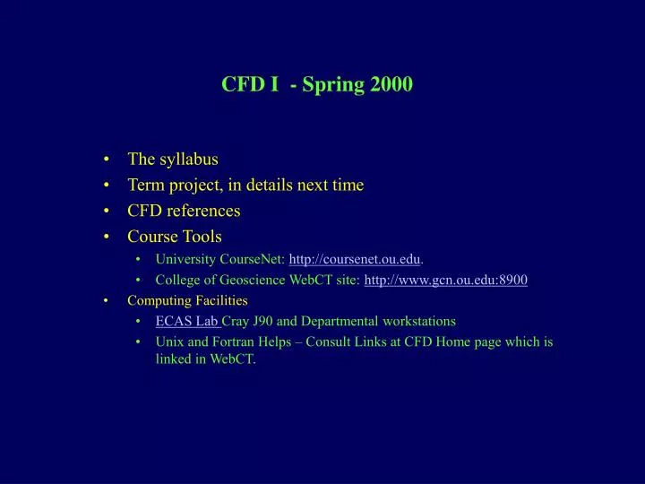
CFD I - Spring 2000. The syllabus Term project, in details next time CFD references Course Tools University CourseNet: http://coursenet.ou.edu . College of Geoscience WebCT site: http://www.gcn.ou.edu:8900 Computing Facilities ECAS Lab Cray J90 and Departmental workstations

E N D
CFD I - Spring 2000 • The syllabus • Term project, in details next time • CFD references • Course Tools • University CourseNet: http://coursenet.ou.edu. • College of Geoscience WebCT site: http://www.gcn.ou.edu:8900 • Computing Facilities • ECAS Lab Cray J90 and Departmental workstations • Unix and Fortran Helps – Consult Links at CFD Home page which is linked in WebCT.
Introduction – Principle of Fluid Motion • Mass Conservation • Newton’s Second of Law • Energy Conservation • Equation of State for Idealized Gas These laws are expressed in terms of mathematical equations, usually as partial differential equations. Most important equations – the Navier-Stokes equations
Approaches for Understanding Fluid Motion • Traditional Approaches • Theoretical • Experimental • Newer Approach • Computational • CFD emerged as the primary tool for engineering design, weather prediction et al, because of the advent of digital computers
Theoretical FD • Science for finding solutions of governing equations in different categories and studying the associated approxiations / assumptions; h = d/2,
Experimental FD • Understanding fluid behavior using laboratory models and experiments. Important for validating theoretical solutions. • E.g., Water tanks, wind tunnels
Computational FD • A Science of Finding numerical solutions of governing equations, using high-speed digital computers
Why Computational FD • Analytical solutions exist only for a handful of typically boring problems • Can control numerical experiments and perform sensitivity studies, some in very ideaized settings. • Can study something that is not directly observable (black holes). • Computer solutions provide a more complete sets of data in time and space • We can perform realistic experiments on phenomena that are not possible to reproduce in reality, e.g., the weather • Much cheaper than laboratory experiments • Much more flexible – each change of configurations, parameters • We can now use computers to DISCOVER new things (drugs, sub‑atomic particles, storm dynamics) much quicker
Positive Internal Shear g=1 Negative Internal Shear g=-1
T=12 Positive Internal Shear g=1 Negative Internal Shear g=-1 No Significant Circulation Induced by Cold Pool
Simulation of an Convective Squall Line in Atmosphere Infrared Imagery Showing Squall Line at 12 UTC January 23, 1999. ARPS 48 h Forecast at 6 km Resolution Shown are the Composite Reflectivity and Mean Sea-level Pressure.
Difficulties with CFD • PDE's are not well‑suited for solution on computers ‑ must approximate a continuous system by a discrete one. One must keep in mind that the governing equations themselves are approximations • Most physically important problems are highly nonlinear ‑ advantage of models is that you can examine the relative contribution of each term. But, how will you then know if the solution is correct? Validation?! • It is impossible to represent all relevant scales in a given problem ‑ there is strong coupling in atmospheric flows and most CFD problems. ENERGY TRANSFERS. (Transparency) • Most of the numerical techniques we use are inherently unstable ‑ often we have to beat down the instability with a hammer, resulting in degraded solutions. We must deal with physical and computational instabilities.
Difficulties with CFD • We often have to impose nonphysical boundary conditions. • We often have to parameterize processes which are not well understood (e.g., rain formation, chemical reactions, turbulence). • The real world is continuous, not discrete. • Often a numerical experiment raises more questions than it answers!!
POSITIVE OUTLOOK • New schemes / algorithms • Bigger and faster computers • Faster network access • Better Desktop computers • Better programming tools and environment • Better understanding of dynamics / predictabilities • etc.