Download
1 / 22
220 likes | 224 Views
This paper explores the use of active learning with the perceptron algorithm, introducing a modified perceptron update and providing bounds on the number of labels required to reach a desired error rate.

E N D
Analysis of perceptron-based active learning • Sanjoy Dasgupta, UCSD • Adam Tauman Kalai, TTI-Chicago • Claire Monteleoni,MIT Dasgupta, Kalai & Monteleoni COLT 2005
Selective sampling, online constraints • Selective sampling framework: • Unlabeled examples, xt, are received one at a time. • Learner makes a prediction at each time-step. • A noiseless oracle to label yt, can be queried at a cost. • Goal: minimize number oflabels to reach error • istheerror rate (w.r.t. the target) on the sampling distribution. • Online constraints: • Space: Learner cannot store all previously seen examples (and then perform batch learning). • Time: Running time of learner’s belief update step should not scale with number of seen examples/mistakes. Dasgupta, Kalai & Monteleoni COLT 2005
AC Milan v. Inter Milan Dasgupta, Kalai & Monteleoni COLT 2005
Problem framework Target: Current hypothesis: Error region: Assumptions: Separability u is through origin x~Uniform on S error rate: u vt t t Dasgupta, Kalai & Monteleoni COLT 2005
Related work • Analysis under selective sampling model, of Query By Committee algorithm [Seung,Opper&Sompolinsky‘92] : • Theorem [Freund,Seung,Shamir&Tishby ‘97]: Under selective sampling from the uniform, QBC can learn a half-space through the origin to generalization error , using Õ(d log 1/) labels. • ! BUT: space required, and time complexity of the update both scale with number of seen mistakes! Dasgupta, Kalai & Monteleoni COLT 2005
Related work • Perceptron: a simple online algorithm: • If yt SGN(vt¢ xt), then: Filtering rule • vt+1 = vt + yt xtUpdate step • Distribution-free mistake bound O(1/2), if exists margin . • Theorem[Baum‘89]: Perceptron, given sequential labeled examples from the uniform distribution, can converge to generalization error after Õ(d/2) mistakes. Dasgupta, Kalai & Monteleoni COLT 2005
Our contributions • A lower bound for Perceptron in active learning context of (1/2)labels. • A modified Perceptron update with a Õ(d log 1/) mistake bound. • An active learning rule and a labelbound of Õ(d log 1/). • A bound of Õ(d log 1/) on total errors (labeled or not). Dasgupta, Kalai & Monteleoni COLT 2005
Perceptron • Perceptron update: vt+1 = vt + yt xt • error does not decrease monotonically. vt+1 vt u xt Dasgupta, Kalai & Monteleoni COLT 2005
Lower bound on labels for Perceptron • Theorem 1: The Perceptron algorithm, using any active learning rule, requires (1/2) labels to reach generalization error w.r.t. the uniform distribution. • Proof idea: Lemma:For small t, the Perceptron update will increase t unless kvtk • is large: (1/sin t).But, kvtk growth rate: So need t ¸ 1/sin2t. • Under uniform, • t/t¸ sin t. vt+1 vt u xt Dasgupta, Kalai & Monteleoni COLT 2005
A modified Perceptron update • Standard Perceptron update: • vt+1 = vt + yt xt • Instead, weight the update by “confidence” w.r.t. current hypothesis vt: • vt+1 = vt + 2 yt|vt¢ xt| xt (v1 = y0x0) • (similar to update in [Blum et al.‘96] for noise-tolerant learning) • Unlike Perceptron: • Error decreases monotonically: • cos(t+1) = u ¢ vt+1 = u ¢ vt+ 2 |vt¢ xt||u ¢ xt| • ¸ u ¢ vt = cos(t) • kvtk =1 (due to factor of 2) Dasgupta, Kalai & Monteleoni COLT 2005
A modified Perceptron update • Perceptron update: vt+1 = vt + yt xt • Modified Perceptron update: vt+1 = vt + 2 yt |vt¢ xt| xt vt+1 vt+1 vt u vt+1 vt xt Dasgupta, Kalai & Monteleoni COLT 2005
Mistake bound • Theorem 2: In the supervised setting, the modified Perceptron converges to generalization error after Õ(d log 1/) mistakes. • Proof idea: The exponential convergence follows from a multiplicative decrease in t: • On an update, • !We lower bound2|vt¢ xt||u ¢ xt|, with high probability, using our distributional assumption. Dasgupta, Kalai & Monteleoni COLT 2005
Mistake bound • Theorem 2: In the supervised setting, the modified Perceptron converges to generalization error after Õ(d log 1/) mistakes. • Lemma (band): For any fixed a: kak=1, · 1 and for x~U on S: • Apply to|vt¢ x| and |u ¢ x| )2|vt¢ xt||u ¢ xt| is • large enough in expectation (using size of t). a k { {x : |a ¢ x| · k} = Dasgupta, Kalai & Monteleoni COLT 2005
Active learning rule • Goal: Filter to label just those points in the error region. • !but t,and thus t unknown! • Define labeling region: • Tradeoff in choosingthreshold st: • If too high, may wait too long for an error. • If too low, resulting update is too small. • makes • constant. • !But t unknown! Choose st adaptively: • Start high. Halve, if no error in R consecutive labels. vt u st { L Dasgupta, Kalai & Monteleoni COLT 2005
Label bound • Theorem 3: In the active learning setting, the modified Perceptron, using the adaptive filtering rule, will converge to generalization error after Õ(d log 1/) labels. • Corollary: The total errors (labeled and unlabeled) will be Õ(d log 1/). Dasgupta, Kalai & Monteleoni COLT 2005
Proof technique • Proof outline: We show the following lemmas hold with sufficient probability: • Lemma 1. st does not decrease too quickly: • Lemma 2. We query labels on a constant fraction of t. • Lemma 3. With constantprobability the update is good. • By algorithm, ~1/R labels are mistakes. 9R = Õ(1). • )Can thus bound labels and total errors by mistakes. Dasgupta, Kalai & Monteleoni COLT 2005
Proof technique • Lemma 1. st is large enough: • Proof: (By contradiction) Let t be first time • Then • A halving event means we saw R labels with no mistakes, so • Lemma 1a: For any particular i, this event happens w.p. · 3/4: Dasgupta, Kalai & Monteleoni COLT 2005
Proof technique Lemma 1a. Proof idea:Using this value of st, band lemma in Rd-1 gives constant probability of x0 falling in appropriately defined band w.r.t. u0. where: x0: component of x orthogonal to vt u0: component of u orthogonal to vt ) vt u st Dasgupta, Kalai & Monteleoni COLT 2005
Proof technique • Lemma 2. We query labels on a constant fraction of t. • Proof: Assume Lemma 1 for lower bound on st. Apply Lemma 1a and band lemma ) • Lemma 3. With constantprobability the update is good. • Proof: Assuming Lemma 1, by Lemma 2, each error is labeled w. constant p. From mistake bound proof, each update is good (multiplicative decrease in error) w. constant p. • Finally, solve for R: Every R labels there is at least 1 update or we halve st, so • There exists R = Õ(1) s.t. Dasgupta, Kalai & Monteleoni COLT 2005
Summary of contributions • samples mistakes labels total errors online? • PAC • complexity • [Long‘03] • [Long‘95] • Perceptron • [Baum‘97] • QBC • [FSST‘97] • [DKM‘05] Dasgupta, Kalai & Monteleoni COLT 2005
Conclusions and open problems • Achieve optimal label-complexity for this problem • unlike QBC, a fully online algorithm • Matching bound on total errors (labeled and unlabeled). • Future work: • Relax distributional assumptions: • Uniform is sufficient but not necessary for proof. • Note: this bound is not possible under arbitrary distributions [Dasgupta‘04]. • Relax separability assumption: • Allow “margin” of tolerated error. • Analyze margin version: • for exponential convergence, without d dependence. Dasgupta, Kalai & Monteleoni COLT 2005
Thank you! Dasgupta, Kalai & Monteleoni COLT 2005