Download

1 / 42
420 likes | 707 Views
Path Analysis. A Brief Intro. Causation. “The search for causal laws is deeply tied up with our subconscious tendency to recreate the universe in our own image.” John Kemeny Something to think about- is the determination of causality a plausible notion?

E N D
Path Analysis A Brief Intro
Causation • “The search for causal laws is deeply tied up with our subconscious tendency to recreate the universe in our own image.” • John Kemeny • Something to think about- is the determination of causality a plausible notion? • Are there genetic determinants of behavior? • Do childhood attributes have a causal relation to adult behavior? • Does smoking cause lung cancer?
Causation • The attempt to determine causal relations among variables requires very deep thinking1 • The topic of causality and its determination is a very old discourse, and very little has been settled • Causality in psychology • You’ll often find that some of the biggest names in psychological science history2 have stopped to ponder the notion of causality explicitly, especially those more methodologically minded
Causation • “Causes are connected with effects, but this is because our theories connect them, not because the world is held together by cosmic glue…The notions behind ‘the cause x’ and ‘the effect y’ are intelligible only against a pattern of theory…” • Hanson • However, while we might be able to find data consistent with a theoretical model, it does not prove that theory or its underlying causal assumptions • Other theoretical models may fit as well or better • It has just not been falsified but merely confirmed • “All models are wrong, but some are useful” • Box
Causal modeling • In the simplest situation of regression, we are behaving as though one variable predicts another • And while some love to say that correlation does not equal causation, there is no assessment of causality with out it • E.g. from Hume1: correlation in time, frequency, space
“Causal Modeling” • Neither statistical technique nor design induce causality in and of themselves • Take the surest of situations- the randomized experiment • Suppose an effect of the treatment is discovered, it may be that • Outliers are an issue, and in such a case the effect is with only a relative few • Even if not outliers, the treatment may not, and likely will not, affect everyone the same way, and while the statistical technique used assumes ‘general’ homogeneity, it does not make it a reality • The model may still be misspecified • The effect is there, but in fact the treatment causes a mediator, which then causes the outcome of interest • One can use any ‘soft’ modeling statistical technique to analyze experimental data • Using regression on experimental data does not detract from its causal conclusion
“Causal Modeling” • Good experimental practice seeks to avoid confounding experimentally manipulated variable with others that might be of influence on the outcome • Sound analysis of observational data would include, and thus control for statistically, confounding factors as well
Causal modeling • With MR for example, the same relationship holds (regardless of variable scale) though the number of variables change, i.e. we still believe some variables are predicting some outcome, which implies a potential causal relationship (whether we want to admit it or not) • In MR, several predictors may be specified to have a causal relationship with the dependent variable • However, the relationship of the predictors among themselves is not causally specified
Identifying causes • Involves: • Theory • Time precedence • Previous research • Logic • Furthermore, in path analysis the cause is almost always deemed probabilistic rather than deterministic • Example: education causes income in the sense that certain jobs are not available to those without one, but one more year of education does not automatically come with its own paycheck
Causal modeling • Given what otherwise would be a typical MR type of situation, if we have a stronger theory to test, we may actually specify predictive relationships among the predictors, we may have more than one DV to examine, or have mediated effects to model • Path analysis allows us to do this
Path Analysis • PA allows for the testing of a model and both direct and indirect effects on some outcome(s) • We have exogenous and endogenous variables • Exogenous • Variation determined by causes outside the model • Ex 1&2 • Endogenous • Variation determined by causes inside the model • En 1&2 • Here we’ll talk of recursive models in which the causal flow goes in one direction • “Recursive” • No causal loops • The path coefficient • That fraction of the standard deviation of the dependent variable for which the designated factor is directly responsible
Basic steps • Think hard about the problem and develop viable model(s) (draw it) • Study relevant literature to find appropriate variables so that you can include common causes of the presumed causes and effects • Not including common causes can have an enormous impact on our conclusions and understanding • Shoe Size Reading Skill • Age causes SS and RS • Possibly the hardest part of path analysis/SEM • Revise the model, prefer lean • Include necessary variables but not every one you could possibly think of • Check identification of the model • Will you have enough information to estimate the model? • Collect reliable data • Must have reliable, valid measures • Estimate the model and assess of fit • Interpret effects • Compare with initial alternative models or others derived via exploration/trimming
Model Identification • A model is identified if it’s theoretically possible to find a unique solution regarding the parameters to be estimated • An eyeball approach: v(v+1)/2 where v is the number of variables; This value, i.e. the number of ‘observations’ in terms of variances and covariances, should be the maximum number of parameters you are trying to estimate • Just-Identified Model • Number of equations is equal to the number of parameters to be estimated • Correlation matrix is reproduced exactly • A model may be just-identified because of constraints imposed and assumptions undertaken by the researcher • Example: simple mediation model
Model Identification • Over-identified • More information than needed to estimate the parameters • Example: V1 V2 V3 (no path between V1 and V3) • 3 correlations but only 2 path coefficients to estimate • That correlation could be reproduced (r13=p32p21) but the model suggests that the effect is only indirect. • An over-identified model may produce more than one estimate for certain parameters, and it too is based on the model imposed by the researcher • Under-identified models contain insufficient information for definite solution for parameters • One will have to impose constraints in order for it to ‘work’ toward a solution • A theoretical problem rather than a statistical one, as paths will have to be deleted or made equal to others
Causality and Identification • While the data may be consistent with the model, that does not make it a valid one, and other models with the same variables might work just as well • E.g. V2 causing both V1 and V3 • Reproduces original correlation r13 • V3 V1 V2; p31 = r13 • Reproduces different correlation for r23 • Gist: whatever the situation, there still is no statistic for causality, no way to prove it with statistics, no way to remove the observer from its estimation. It is still our theory which guides us.
What variables to include • No straightforward answer • Want a not too complex model that includes the ‘most’ relevant variables, but that is not too simplistic either • On the technical side, including unreliable measures will only hurt the model • Also collinearity may cause problems as the program essentially tries to solve for identical variables
Directionality • Given the gist of what constitutes a causal relationship, many causes will be clear and direction obvious • In cases where it still might be unclear consider: • The conceptualization of the construct(s) may need reworking • The specifics of the population of interest/data collection procedure may suggest a specific direction that might not hold for other research situations • Forgo path analysis for multiple or multivariate regression • As part of the analysis compare models with different directionalities • Include reciprocal effects
Method • While MR can be used and some of how it is discussed here relate PA to MR, most likely you will use Maximum Likelihood1 • ML will require an appropriate package, and will produce different results as it uses mathematically intensive methods to estimate the all the parameters simultaneously, and provides goodness of fit measures that the MR approach will not • For just-identified2, recursive models, the MR and ML approaches provide the same path coefficients, and will typically be similar for large sample over-identified models
Assumptions • The maximum likelihood approach has most of the same assumptions but there are exceptions • Linear relations among variables, additive and causal • No reverse causation • Residuals1 not correlated with the variables that precede it or with each other • e3 not correlated with 1 & 2 • e4 not with 1,2,3 • Other assumptions of regression analysis hold • If relying on statistical test probabilities, continuous variables now require multivariate normality • Rather than just normality of residuals as in MR
Relevant equations for this model assuming variables are in standard scores V1 standardized = z1 z1 = e1 z2 = p21z1 + e2 z3 = p31z1 + p32z2 + e3 z4 = p41z1 + p42z2 + p43z3 + e4 e3 e4 V1 p41 p31 p21 p43 V3 V4 p32 p42 e2 V2 Example Equations
Obtaining a path coefficient • Recall the formula for r • Substitute in z2 from the equation from the previous slide • But, the first part after p21 is just the variance for the first variable, and since it’s standardized it equals 1. The second part is assumed to be zero (i.e. residuals are independent of the predictor). So… • The path coefficient = r whenever a variable has a single cause and residual • The same thing you saw for the standardized coefficient in simple regression
Multiple causes • What about multiple causes? • Though typically estimated differently, the path coefficients for standardized data are equal to the beta coefficients one would find from a regression • E.g. of variable 3 on its causes, variables 1 and 2 • The error variance, or disturbance is just like in any regression, 1 – R2 for that variable regressed on its causes1 • Similarly for variable 4, the coefficients would represent the standardized coefficients from its being regressed on its three causes • Note that for non-recursive models p12≠ p21
The tracing rule: The correlation between two variables X and Y is equal to the sum of the product of all paths from each possible tracing between X and Y Or another way to put it, the sum of the product of each path from all causes of Y and the correlation of those causes with X Path coefficients and correlation
Interpretation of the path coefficient • Same as standardized coefficient in regression as we are talking about standardized data • One can leave in raw form when dealing with meaningful scales • Again, they more generally they imply a weak causal ordering • Not that X causes Y but that if X and Y are causally related it goes in that direction and not the reverse
Decomposing correlations • Note the two predictor example in a regular regression in which the predictors are exogenous and correlated • What would be the correlation of variable 1 and 3? • It comes from the direct effect but also has correlated causes • p31 is the direct effect • r13 – p31 is that unanalyzed portion due to correlated causes • r13 = p31 + r12p32
Mediated causes1 Total effect of V1 on V3 is r13 r13 = p31 + p21p32 Total effect = direct effect + indirect effect As discussed before, the mediated (indirect) effect is the change in the correlation between two variables when the mediator is added to the model in this simple setting p21*p32 = r13- p31 Mediation
More complex • Example of decomposition of 2 correlations from the following model • r14 = p41 + p31p43 + r12p42 + r12p32p43 • r34 = p43 + p41p31 + p42p32 + r12p42p31 + r12p32p41 • Direct effect • Indirect Effect • Spurious Effect (effects due to common causes)
The point: Fit • Since we can decompose the correlations, once coefficients are chosen we can reproduce (predict) the correlation matrix based on our estimated parameters (path coefficients) • With just-identified models the correlations are reproduced exactly • With over-identified models, some measures of Goodness of Fit look at how well we are able to reproduce the correlation matrix
Effects • To summarize, a correlation may be decomposed into direct effects, indirect effects, unanalyzed effects, and spurious effects (due to common causes) • What’s interesting to point out is that while the direct effect of a variable on some other may not be noticeably large, it’s total effect may be interesting (total = direct +indirect)
Theory trimming • Model Respecification • One may perform significant tests for path coefficients, same as in MR, for the various regression equations appropriate to the model • Perhaps ‘trim’ non-sig paths • However, the same issues apply as we have had with other analyses • Sample size • Sampling variability • Furthermore, the test of coefficients do not equate a test of the model itself • “If we look over the phenomena to find agreement with theory, it is a mere question of ingenuity and industry how many we shall find” • C.S. Peirce • One should consider the practical meaningfulness of the coefficient within the context of the model specified by theory
Family Background Essentially SES Ability Aptitude, Previous Achievement Motivation Intrinisic, perserverance Coursework How much time spent in instruction, opportunity for learning Achievement A measure of learning Academic Coursework Ability Achievement Family Background Motivation Example Model
Data • FB Ab Mot Cou Ach • Family Back 1 • Ability .417 1 • Motivation .190 .205 1 • Coursework .372 .498 .375 1 • Achieve .417 .737 .255 .615 1
d2 .807 d1 Academic Coursework .9091 .374 .310 Ability .267 .551 .609 Achievement .417 d3 .069 Family Background .152 .013 Motivation .127 .972 d4 Example Model
Effects • Example for motivation • Direct = .013 • Indirect = .267*.310 = .083 • Further back in the model it gets more complicated • Ability • Direct = .551 • Indirect through coursework = .374*.310 = .116 • Indirect through motivation = .152*.013 = .002 • Indirect through motivation then coursework = .152*.267*.310 = .013
Total effects • Doing a sequential regression, we can see the total effects (bold)1 • Start with the exogenous variable and move in the direction of the flow from there
“Goodness of fit” • How well does the data as a whole agree with the model? • There are numerous fit indices, and numerous debates regarding them • Issues with all measures: • Parts of the data may in fact have poor fit while overall fit is ok • Does not indicate theoretical meaningfulness • Do not indicate predictive power
Goodness of fit • X2 test • Is really a badness of fit index, and in general terms, is testing your model against one which would fit the data perfectly (a just-identified model) • Sample covariance/correlation matrix vs. reproduced • df = the difference between the # of parameters and correlations used to estimate them • In this case, you are hoping not to reject • If you do, it suggests you need to add some variable to the model • The problem with this approach entails all the same issues of any test of statistical significance • Sample size, assumptions etc. • Furthermore, one cannot accept a null hypothesis from an NHST approach • Thought that doesn’t stop a lot of people
Goodness of fit • Root mean square residual • As the name implies, a kind of average residual between the fitted and original covariance matrix • Like covariance itself, hard to understand its scale • Standardized (regarding the correlation matrix) it ranges from 0-1 • 0 perfect fit • Goodness of Fit Index, Adjusted GFI1 • Kind of like our R2 and adjusted R2 for the structural model world, but a bit different interpretation • It is the percent of observed covariances explained by the covariances implied by the model • R2 in multiple regression deals with error variance whereas GFI deals with error in reproducing the variance-covariance matrix • Rule of thumb: .9 for GFI, .8 for adjusted, which takes into account the number of parameters being estimated • Incremental fit indices • Bentler’s Normed Fit Index, Non-Normed FI (Tucker-Lewis Index), and CFI (NFI adjusted for sample size) test the model against an independence model • E.g. 80% would suggest the model fits the data 80% better • Others Akaike Information Criterion, Bayesian Information Criterion • Good for model comparison1, can work for non-nested models also
Model Exploration • If specification error is suspected, one may examine other plausible models statistically • However, it is generally not a good idea to let the program determine these alternative models as ‘Modification Indices’ can vary wildly even with notably large datasets • A much better approach is to go into the analysis with multiple theoretically plausible models to begin with, and assess relative fit • One may also take an exploratory approach from the outset, however this, like any other time, would require some form of validation procedure
Extensions • Nonrecursive models • Bicausal relationships, Feedback loops • Require special care for identification and still may be difficult to pull off • Multiple group analysis • Do parameter estimates vary over groups? • In other words, do these predictors interact with a grouping variable? • Partial Least Squares • We did it for regression but it can be extended to multiple outcomes/SEM • Software
R example: library(sem) data <- read.moments(diag=FALSE, names=c('FamilyBackgroud', 'Ability', 'Motivation', 'Coursework', 'Achievement')) .417 .190 .205 .372 .498 .375 .417 .737 .255 .615 model <- specify.model() FamilyBackgroud -> Ability, gam11, NA FamilyBackgroud -> Motivation, gam21, NA Ability -> Motivation, gam22, NA FamilyBackgroud -> Coursework, gam31, NA Ability -> Coursework, gam32, NA Motivation -> Coursework, gam33, NA FamilyBackgroud -> Achievement, gam41, NA Ability -> Achievement, gam42, NA Coursework -> Achievement, gam43, NA Motivation -> Achievement, gam44, NA Ability <-> Ability, psi1, NA Motivation <-> Motivation, psi2, NA Coursework <-> Coursework, psi3, NA Achievement <-> Achievement, psi4, NA path.model <- sem(model, data, 1000, fixed.x='FamilyBackgroud') summary(path.model)
Path Analysis • Rest assured, ‘causal modeling’ no more ‘proves’ causality than any other statistical technique • What path analysis does provide however is a more intricate way of thinking about testing our research problem • Use all the available information, as well as your own intuition, to come to a global assessment about the nature of the various relationships among the variables of interest