Download
1 / 17
170 likes | 263 Views
HL-RDHM, STAT_Q, XDMS Overview and General Features. Lecture 3. Lecture/Workshop Approach. Lectures 3, 4, and 5 are intended to provide scientific, and technical background and introduce the workshops

E N D
HL-RDHM, STAT_Q, XDMS Overview and General Features Lecture 3
Lecture/Workshop Approach • Lectures 3, 4, and 5 are intended to provide scientific, and technical background and introduce the workshops • Details not covered in lecture are covered in the HL-RDHM 2.0 User’s Manual and other documents • Workshops are scripted to make sure the full range of software capabilities are described given the short time we have; once a script is completed, we encourage individual experimentation with any remaining time • THIS IS THE FIRST TIME WE’VE GIVEN THIS COURSE! WE DON’T KNOW HOW LONG THINGS WILL TAKE. WE WILL TRY TO ADJUST TIMES AS NEEDED
Outline • What are HL-RDHM, DHM, XDMS, and STAT_Q? • HL-RDHM Overview • Using ICP Plot-TS, STAT_QME with HL-RDHM time series files • STAT_Q Overview • XDMS Overview (James Paul) • DHM Overview will be given by Lee Cajina
Acronyms and Features Evolution Core Distributed Model Research Track HL-RMS (Koren, 2004) HL-RDHM (Research model shared as AWIPS local application) DHM (AWIPS operational software) DMS 1.0 (ABRFC, WGRFC prototype) Operational Track Complementary Programs XDMS: GUI for grid and time series display developed at ABRFC Stat_Q: Stand-alone statistical analysis program developed at OHD for analyzing time series data in NWSRFS Calibration System DATACARD Format.
Typical RFC Forecast Basin Modeling Procedure Step Available Tool HL-RDHM Simulation/Calibration Mode Calibrated scalars, Initial states DHM Forecast Mode
HL-RDHM 2.0 Features • Designed for river forecast, flash flood, and water resources research and development • Supports gridded connected or unconnected domain runs • Flexible I/O in standard NWS formats • Common programming framework for researchers • Facilitates rapid model testing • Promotes good (modular) programming • Multiple modeling resolutions • Contains models for all hydrologic cycle components: snow, rainfall/runoff, frozen ground, overland and channel routing • Simulation/calibration mode exists. Forecast mode planned for HL-RDHM 2.1.
HL-RDHM Generic Computational Flow Chart • Researcher defines functions for 1-3 of the gray rectangles. System handles many tedious I/O tasks. • HL-RDHM Developer’s Manual available for download on the LAD
HL-RDHM 2.0 Available Operations • Snow-17 (snow17) • SAC-SMA-HT (sac, calsac*) • Continuous API (api) • Frozen ground (frz) • Overland and channel routing (rutpix7,rutpix9,calrutpix7,calrutpix9) • Automatic optimization (funcOpt) * Operations preceded by the ‘cal’ prefix are coded to improve performance over the non-’cal’ version. These operations are particularly useful for automatic and manual calibration runs. The non-‘cal’ versions have their own advantages (e.g. more output options and developer flexibility). Cal and non-cal operations cannot be mixed.
Default Parameter Files Provided with HL-RDHM 2.0 XMRG file format hrapfa10.xmrg**: flow accumulation grid for display in XDMS (not used by HL-RDHM) hrapfd10.xmrg**: flow direction grid for display in XDMS (not used by HL-RDHM) xxrfc4k.con: ASCII connectivity files (one for each CONUS RFC) * Grid is a template and requires local customization. ** All grids cover CONUS with the exception of rutpix_SLOPH, rutpix_SLOPC, rutpix_SLOPC1, hrapfa10.xmrg, and hrapfd10.xmrg which are provided separately to each CONUS RFC
Key Words • Key words are used to define a model run in the Input Deck (ASCII file) • User Manual Chapter 8 describes all key words and syntax specifics Selected Key Words • time-period • time-step • connectivity (used for a connected domain) • window-in-hrap (used for an unconnected domain) • subwindows • output-path • input-path • ignore-1d-xmrg • operations • window-input • input-data (specify parameters or scale factors for specific basins) • mask (a grid defining an irregular domain boundary for unconnected calculations can be provided)
Outputs • Output Key Words • output-grid-before-timeloop • output-grid-inside-timeloop • output-grid-after-timeloop • output-grid-step • output-grid-last-step • output-timeseries-basin-average • output-timeseries-basin-outlet • Can output grids or time series for any model states in selected operations (102 different states for all operations) • Can output grids for any parameters in selected operations (136 different parameters for all operations) • Output Formats • Grids are output as XMRG-like binary files • Time series are output in NWSRFS Calibration System DATACARD format • XDMS displays these grids and time series • ICP displays these time series
Example HL-RDHM Input Deck #basin id and factors for input data # basin id followed by "name=value" pairs #------------------ #----- TALO2 ------ #------------------ input-data = TALO2 #SAC parameters input-data = sac_PCTIM=0.005 input-data = sac_ADIMP=0.1 input-data = sac_RIVA=0.03 input-data = sac_EFC=0.5 input-data = sac_SIDE=0.0 input-data = sac_RSERV=0.3 input-data = sac_UZTWM=-0.5 input-data = sac_UZFWM=-0.80 input-data = sac_UZK=-0.7 input-data = sac_ZPERC=-3.49 input-data = sac_REXP=-0.74 input-data = sac_LZTWM=-0.82 input-data = sac_LZFSM=-1.24 input-data = sac_LZFPM=-2.1 input-data = sac_LZSK=-0.51 input-data = sac_LZPK=-0.45 input-data = sac_PFREE=-0.30 input-data = pe_JAN=0.9 pe_FEB=1.0 pe_MAR=1.70 input-data = pe_APR=2.7 pe_MAY=3.7 pe_JUN=5.2 input-data = pe_JUL=5.6 pe_AUG=5.3 pe_SEP=4.1 input-data = pe_OCT=2.4 pe_NOV=1.3 pe_DEC=1.0 input-data = peadj_JAN=1.0 peadj_FEB=1.0 peadj_MAR=1.0 input-data = peadj_APR=1.0 peadj_MAY=1.0 peadj_JUN=1.0 input-data = peadj_JUL=1.0 peadj_AUG=1.0 peadj_SEP=1.0 input-data = peadj_OCT=1.0 peadj_NOV=1.0 peadj_DEC=1.0 #SAC states input-data = uztwc=0.66 uzfwc=0.0 lztwc=0.69 input-data = lzfsc=0.0 lzfpc=0.57 adimpc=0.69 #rutpix parameters input-data = rutpix_Q0CHN=-1.8 rutpix_QMCHN=-0.92 #rutpix states input-data = areac=5.0 depth=0.0 #simulation time period time-period = 19951001T00 20060930T23 # ignore-1d-xmrg = false #simulation time step in the format of HH:MM:SS.XXXX time-step = 1 #the connectivity file connectivity = /fs/hsmb5/hydro/rms/sequence/abrfc_var_adj2.con #output path output-path = /fs/hsmb5/hydro/dmip2/talo2/ws1a #input paths input-path = /fs/hsmb5/hydro/rms/parameterslx input-path = /fs/hsmb5/hydro/Hydro_Data/ABRFC/PRECIPITATION #selected operations operations = calsac calrutpix9 #data to be output before, inside and after timeloop in grid format #In number of timestep, example, 2 means output every 2 timestep #output-grid-step = 1 #output-grid-before-timeloop = sac_LZFPM #data to be output at the last time step #output-grid-last-step = uztwc uzfwc lztwc lzfsc lzfpc adimpc #output-grid-last-step = real_uztwc real_uzfwc real_lztwc real_lzfsc #output-grid-inside-timeloop = discharge surfaceFlow #Time series to be averaged over every basin #output-timeseries-basin-average = xmrg #output-timeseries-basin-average = surfaceFlow #Time series at the outlet output-timeseries-basin-outlet = discharge
TALO2 , analize results 10 1996 9 2006 DEF-TS TALO2 QIN 1 INPUT ws1a/talo2.mod2 TALO1 SQIN 1 INPUT ws1a/TALO2ap_discharge.outlet_ts TALO2 SQIN 1 INPUT ws1a/TALO2_discharge.outlet_ts TALO2 MAPX 1 INPUT ws1a/TALO2_xmrg.ave_ts TALO2 QME 24 INTERNAL TALO1 SQME 24 INTERNAL TALO2 SQME 24 INTERNAL END MEAN-Q TALO1 TALO1 SQIN 1 TALO1 SQME 24 MEAN-Q TALO2 TALO2 SQIN 1 TALO2 SQME 24 MEAN-Q TALO2-OBS TALO2 QIN 1 TALO2 QME 24 PLOT-TS TALO2 SCE vs. RFC 3 2 4 0 ARIT 30 0.0 50.0 1 TALO2 MAPX 1 pcp P ARIT 30 0.0 1000.0 3 TALO2 QIN 1 USGS o TALO1 SQIN 1 u u TALO2 SQIN 1 c c STAT-QME TALO1 Illinois - uncali 2483. TALO1 SQME 24 TALO2 QME 24 1 QUAR STAT-QME TALO2 Illinois - calib 2483. TALO2 SQME 24 TALO2 QME 24 1 QUAR STOP Example ICP Input Deck to Display HL-RDHM time series
Stat_q • Statistical analysis of any two time series in single column NWSRFS Calibration Data Card format • Similar to STAT_QME but with many more options • Flexible analysis time step (hourly – 24 hourly) • Yearly, monthly statistical summaries • Flow interval statistics • Event statistics for user defined events
GIS Import/Export Tools Utilities will be made available to export grids or import grids in ESRI gridascii format. Format can also be easily imported to GRASS software. • xmrg2asc • asc2xmrg
Workshops Overview • Workshop 1: Become familiar with HL-RDHM, XDMS, ICP, and STAT-Q. Step through some examples to demonstrate basic HL-RDHM simulation mode features, use of XDMS to examine spatial output, and use ICP and STAT-Q to examine time series outputs. • Workshop 2: Step through procedures for local routing parameter customization (HL-RDHM User’s Manual Chapter 9) • Workshop 3: Run through a simple automatic calibration exercise. Examine hydrograph results in ICP before and after calibration. Manually examine the impacts of parameter scalar changes for both rainfall-runoff and routing. • Workshop 4: Setup and run DHM through IFP. • Workshop 5: Demonstrate an uncalibrated run over a large area. Revisit any questions from earlier workshops. Continue Workshop 4 if necessary. Workshops assume some basic knowledge of existing RFC software applications such as IFP and ICP. Therefore let’s try to put at least one experienced RFC person in each group.
Workshops Overview ABRFC KNSO2 WTTO2 TALO2 Workshop exercises will focus on the ABRFC domain with most specific examples coming from the Illinois River above Tahlequah (TALO2) and two subbasins (The Illinois R. at Kansas (KNSO2) and the Illinois R. at Watts (WTTO2))