Astrometry

4. Astrometry

5. Check that the image is correct from the point of view of astrometry. It is assumed that you know the rough centre, orientation and image scale.

6. Check that the image is correct from the point of view of astrometry. It is assumed that you know the rough centre, orientation and image scale. The next stage is to get some reference positions from an on-line catalogue.

7. Check that the image is correct from the point of view of astrometry. You should get a list of positions that are displayed as circles with interior crosses over your image.

8. Check that the image is correct from the point of view of astrometry. You should get a list of positions that are displayed as circles with interior crosses over your image. If you're good or lucky then you should be able to spot the pattern between the catalog positions and your image.

9. Check that the image is correct from the point of view of astrometry. You should get a list of positions that are displayed as circles with interior crosses over your image. If you're good or lucky then you should be able to spot the pattern between the catalog positions and your image. The next stage is to use these positions to fit a proper solution: drag the magenta circles in the right positions.

10. Light curves

11. How is a specific source discovered? (TDE, SN, etc)

15. Spectral energy distributions (SEDs)

16. Spectrum and spectral energy distribution

18. Spectral energy distributions for typical galaxies - an old elliptical galaxy, two types of spiral galaxies (Sb in green and Sd), an AGN (Markarian 231, solid black), a QSO (dotted black), and a merging and star-bursting galaxy Arp 220.

19. For a starbursting galaxy that is undergoing a merging event, such as Arp 220 (purple line), the SED shows that the galaxy is very bright in the infrared compared to its optical emission and compared to normal star-forming galaxies like the two spiral galaxies. That is why Arp 220 belongs to the class of ultra-luminous infrared galaxies.

20. AGN on the other hand show themselves in the ultraviolet, optical, X-ray, and sometimes also at radio wavelengths. The overall shape of an AGN SED (shown here is that of Mrk 231) is similar to that of a power law, meaning the black line is very flat at optical and IR wavelengths. The SED of a QSO, a quasi stellar object, an object for which the AGN outshines the host galaxy in which it resides, is very steep and shows emission lines in the UV and optical.

21. If dust is present in a galaxy then some of the ultraviolet and blue optical light is absorbed and re-emitted in the infrared which can be seen as bumps in the purple, blue and green curves (around a wavelength of 5 to 110 micron). You might have also noticed the "spikes" of emission in the SEDs around about 5 to 12 micron, these are caused by so-called polycyclic aromatic hydrocarbons (PAHs), which are a class of organic molecules. They give important clues towards the structures of dust in galaxies, star formation, and the merger histories of galaxies.

22. Emitting sources and emission processes at different wavelengths

23. Diagrams • There is a relationship between the luminosity & surface temperature based upon: • the initial mass of a star • its age • its composition (usually a small effect)

24. H-R diagram (L-T)

25. H-R diagram (L-Spectral classes)

26. To first order, the light emitted by a star is a black body. Thus, rather than actually measure & plot (in Kelvin) the temperature of every star, it is MUCH easier and quicker to simply measure & plot the ratio of the intensity of the star in two spectral bands. This ratio is then directly related to the black body function and hence temperature. For primarily historical reasons, the ratio is usually expressed as the difference (in magnitudes) between two standard (optical/IR) spectral bands and is known as the color. Traditionally, the most commonly used color is the difference between the B and V bands (centered at 440 & 550 nm, respectively) and usually written as simply B – V.

27. Similarly, rather than actually measure & plot (in W/m^2) the total flux of every star, it is MUCH easier to simply measure & plot the flux in a standard spectral band. Again since the emitted spectra are black bodies, this is directly related to the total flux. Traditionally, the most commonly used band is the V band (550 nm) and usually written as simply V.

28. Hence, typically CM diagrams are used rather than HR diagrams. For example - if the distances to all the stars have been determined, then this might be a plot of B -V versus absolute V band magnitude. - if the distances to all the stars have NOT been determined (say for a star cluster), then this might be a plot of B - V versus apparent V band magnitude. These are both equivalent to plots of luminosity vs. temperature.

29. In order to compare CM diagrams of two different clusters at two different distances, you need to know the distance to each cluster in order to calculate the absolute magnitude from the apparent magnitude.

30. In order to compare CM diagrams of two different clusters at two different distances, you need to know the distance to each cluster in order to calculate the absolute magnitude from the apparent magnitude. But what if you don't know the distances to the clusters? Wouldn't it be nice to still be able to learn something about the clusters, even if you don't know the distances?

31. The magnitude of a star is related to the log of the flux. Therefore, a color (or the difference of two magnitudes) is related to the ratio of the fluxes. When you take the ratio of the fluxes of the same star, the distance cancels out.

32. The magnitude of a star is related to the log of the flux. Therefore, a color (or the difference of two magnitudes) is related to the ratio of the fluxes. When you take the ratio of the fluxes of the same star, the distance cancels out. The point is that colors are independent of distances! So a color-color plot is also independent of distance.

33. The magnitude of a star is related to the log of the flux. Therefore, a color (or the difference of two magnitudes) is related to the ratio of the fluxes. When you take the ratio of the fluxes of the same star, the distance cancels out. The point is that colors are independent of distances! So a color-color plot is also independent of distance. Example: by studying main-sequence clusters, we can determine the locations of "normal" stars (or other objects) in nearly any color-color space. Then, stars (or other objects) that have colors different than these normal objects stand out.

34. The relationship between two colors (U-V and V-I) for normal stars is indicated by the line marked "ZAMS Relation." Normal stars are clumped along this line. Stars significantly above this line are brighter than expected in U-V given their observed color in V-I.

35. Color-color plots can be used to separate objects of different types, such as distinguishing galaxies from stars.

36. i*-z* and z*-J color-color diagram How the quasars (lower right) are different than brown dwarfs (top) and more boring objects (cluster of points). T dwarf L dwarf Quasar BAL quasar http://iopscience.iop.org/article/10.1086/324111/pdf

37. i*-z* and z*-J color-color diagram How the quasars (lower right) are different than brown dwarfs (top) and more boring objects (cluster of points). T dwarf L dwarf Quasar BAL quasar http://iopscience.iop.org/article/10.1086/324111/pdf

38. i*-z* and z*-J color-color diagram How the quasars (lower right) are different than brown dwarfs (top) and more boring objects (cluster of points). T dwarf L dwarf Quasar BAL quasar http://iopscience.iop.org/article/10.1086/324111/pdf

39. i*-z* and z*-J color-color diagram How the quasars (lower right) are different than brown dwarfs (top) and more boring objects (cluster of points). T dwarf L dwarf Quasar BAL quasar http://iopscience.iop.org/article/10.1086/324111/pdf

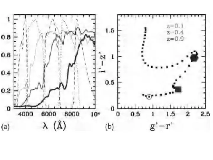
40. SDSS The Sloan Digital Sky Survey has created the most detailed three-dimensional maps of the Universe ever made, with deep multi-color images of one third of the sky, and spectra for more than three million astronomical objects. eBOSS (Extended Baryon Oscillation Spectroscopic Survey) will map the distribution of galaxies and quasars from when the Universe was 3 to 8 billion years old, a critical time when dark energy started to affect the expansion of the Universe. eBOSS concentrates its efforts on the observation of galaxies and in particular quasars, in a range of distances (redshifts) currently left completely unexplored by other three-dimensional maps of large-scale structure in the Universe. In filling this gap, eBOSS will create the largest volume survey of the Universe to date.

41. SDSS: camera and filters The Sloan Digital Sky Survey has created the most detailed three-dimensional maps of the Universe ever made, with deep multi-color images of one third of the sky, and spectra for more than three million astronomical objects. SDSS camera The imaging camera collects photometric imaging data using an array of 30 SITe/Tektronix 2048 by 2048 pixel CCDs arranged in six columns of five CCDs each, aligned with the pixel columns of the CCDs themselves. SDSS r, i, u, z, and g filters cover the respective rows of the array, in that order.