Download

1 / 29
290 likes | 377 Views
Alternative PK microeconomic foundations. The firm: Costing and Pricing. A key feature of most firms. Firms hold excess capacity, or reserve capacity; They can (nearly) always produce more. Why is there ‘excess capacity’?.

E N D
Alternative PK microeconomic foundations The firm: Costing and Pricing
A key feature of most firms • Firms hold excess capacity, or reserve capacity; • They can (nearly) always produce more.
Why is there ‘excess capacity’? • 1. Excess capacity is a deterrent to entry by new or outside firms (Sylos Labini). • 2. A reserve of capacity is necessary to take care of possible shifts in the pattern of demand (Steindl 1952). • 3. Fear of losing share of market when demand suddenly rises. • 4. Indivisibility of plants. • 5. A range of acceptable rates of capacity utilization (Dutt (1990)
The definition of practical capacity • Each firm usually has a number of physical plants, which are generally divided into a number of segments or assembly lines. • The level of practical capacity is defined as the production capacity of a plant or plant segment, as measured by engineers, the so-called engineer-rated capacity (Eichner, 1976, p. 62). • Or as “the output achieved with normal length of working time, with sufficient shut-downs to allow for repairs and maintenance, and without disturbance in the smooth running of the production process” (Steindl, 1952, p. 7).
Stylized facts of costing • Marginal costs (or direct or prime unit costs) are constant up to practical capacity (fixed technical coefficients) • These include wages, raw material costs and intermediate goods costs that directly enter production • Total unit costs (direct and indirect unit costs) are decreasing up to practical capacity • These include standard fixed costs, but also all overhead or indirect costs, including general shop and enterprise expenditures, as well as supervision costs, transportation costs, etc. • Full capacity is defined as the sum of practical capacity of all plants • It is possible to produce beyond total capacity, up to theoretical capacity, but at rising unit costs • Firms usually operate at 70 to 90% of full capacity
The shape of cost curves MC UC UDC AVC = UDC = MC q qfc qth
How capacity utilization is computed • In Canada, Statistics Canada, the national statistical agency, carries out an annual survey (the Capital and Repair Expenditures Survey) where they ask 7,000 companies regarding their capacity utilization rates. • In surveying these firms, they ask the following question: “For [2008], this plant has been operating at which percentage of its capacity?” • The survey specifies that “Capacity is defined as maximum production attainable under normal conditions”, by taking into account regular holidays.
Statistics Canada’s examples. • “Plant ‘A’ normally operates one shift a day, five days a week and given this operation pattern, capacity production is 150 units of product for the month. In that month, actual production was 125 units. The capacity use rate for plant ‘A’ is (125/150) * 100 = 83%.” • “Now suppose that plan ‘A’ had to open for a shift on Saturdays to satisfy an abnormal surge in demand for its product. Given this plant’s normal operation schedule, capacity production remains at 150 units. Actual production has grown to 160 units, so capacity use would be (160/150) * 100 = 107%.”
The Alan Blinder (1998) survey of U.S. firms • 10% of respondents say marginal costs are rising (a result also obtained by Fogg 1956) • 40% say they are falling • 50% say they are constant • Although the question mentioned « variable costs of producing more units », there may have been some confusion between unit direct costs and total unit costs, or else overhead labour costs may have been included into variable costs (cf. Yordon 1987).
p UC MC p .NUC NUC .UDC UDC q qs qfc qth 80% 100%
The relationship between sales and the profit share • When sales are higher, the realized net profit margin will be larger. • In other words, the net profit share of the firm will be higher
Variants of cost-plus pricing • 1. Simple mark-up pricing (Kalecki) p = (1+)(UDC) , UDC=W/pr • 2. Historic full cost pricing (Godley) p = (1+)(EHUC) • 3. Normal cost pricing (Andrews) p = (1+)(NUC) • 4. Target-return pricing (Lanzillotti, GM) = rnv/ (un – rnv)
Historic full cost pricingp = (1+)(EHUC) • Historic full cost pricing takes into consideration the fact that goods sold this period are in part taken out of stocks of inventories, that is, goods that were produced in the previous period at the unit cost: UDC-1, • The rest of what is being sold has been produced this period, at the current cost UDC. • To set prices firms must make estimates of sales (se); they don’t know the proportion of sales that will arise out of inventories. Call this proportion: • σse = in-1/se • EHUDC, the expected historic direct costs will thus be: • EHUDC = σse.UDC-1 + (1 - σse).UDC
Historic full cost pricing (2) • To the direct costs, Godley adds the interest costs on inventories, to get EHUC: • EHUC = (1 - σse).UDC + σse (1 + r).UDC-1 • Ultimately, putting together these equations, the price equation, assuming full-cost historic pricing, is given by: p = (1+)(EHUC) • p = (1 + ){(1 - σse).UDC + σse (1 + r).UDC-1} • With cost inflation, the formula becomes: • p = (1 + ){(1 + σse.rr).UDC} • where rr is the real rate of interest, the nominal rate being deflated by the rate of cost inflation.
Normal cost pricing • With normal cost pricing, normal unit costs are computed. These are costs computed as if normal ratios were achieved. They are thus simpler to handle. One need not know what is the current inventories to sales ratio • The normal inventories to sales ratio is the target rate set by firms, σT = inT/s • It follows that normal direct costs are: • NDC = (1 - σT).UDC + σT.(1 + r).UDC-1 And hence: p = (1+)(NUC) • p = (1 + ){(1 - σT).UDC + σT.(1 + r).UDC-1} • With cost inflation, the formula becomes: • p = (1 + ){(1 + σT.rr).UDC}
Target-return pricing (Lanzillotti, GM)p = (1+)(NUC) = rsv/ (us – rsv) • Target-return pricing is the industrial- organization equivalent of Sraffian pricing. • The only major difference is that the target rates of return rsare assumed to be uniform (identical) in Sraffian pricing.
Prices of production and target return pricing • The Sraffian prices of production (see Pasinetti, 1977), excluding intermediate goods, • p = wn + rMp • pis a column-vector of prices, w is the wage rate, nand M are a vector and a matrix of technical coefficients representing respectively labour per unit of output and the amounts of each kind of machines per unit of output). Finally, r is the uniform profit rate. • We can re-write the above equation: • p = wn [I – rM] -1 • This equation is very similar to target-return pricing in the case of the simple firm. By integrating the value of Θ in the normal-cost pricing equation, and assuming that direct costs are wages per unit of production, we get: • p = unw.n (un – rn.v) -1
Target return pricing or the determinants of the costing margin or normal profit rate rs • Check: • p = (1+)(NUC) • = rsv/ (us – rsv) • Use: r = i + g/(1+) • Higher target rates are induced by: • Faster growth rates • Higher real interest rates • Tougher borrowing requirements (low )
Implications • Cost-plus pricing shows clearly that the purpose of pricing is income distribution • Income distribution is at the heart of inflation phenomena • Higher demand does not necessarily induce higher prices or higher inflation rates • Cost inflation may be induced by energy and material world price increases
Further implications, for the incidence of the corporate tax • In the competitive model, the tax on corporate profits has no incidence on prices, since it has no effect on marginal costs and hence on the supply curve. • Similarly, in the monopoly model, once again the tax on corporate profits has no incidence on prices. Hence in these two cases, the corporate tax falls entirely on owners. • In the cost-plus model, in particular the target-return pricing model, corporations will shift the tax onto consumers, by pushing up the profit margin and prices.
Some questions about cost-plus pricing… • Isn’t there some firms that have more efficient plants? PC1 PC2 PC3 FC
Isn’t this rising marginal costs? • When they reduce production, firms do not necessarily close down the least efficient plants. A general reduction in demand will be met closing down segments of all plants, rather than closing down all segments of the least efficient plant
A similar objection at the industry level: Do the least efficient firms close down? • No, high-cost firms and low-cost firms can compete. When demand falls, the reduction in output is spread proportionately over all firms. • When demand expands, unit costs for each firm go down, and hence “productivity rises because the rise in output following the rise in demand is shared among all firms, not concentrated among the marginal firms” (Kaldor 1985, p. 47).
The elimination of high-cost firms is a long-run affair • Firms that have have high costs can still make profits, but their profit rates will be lower than those of the low-cost firms. • As a result, these high-cost firms face a more stringent expansion frontier. Because they face a finance frontier, they will be unable to grow as fast, and hence their share of the market will gradually vanish.
Low-cost vs high-cost firms and the expansion frontier Profit rate R Finance Frontier r G Low-cost firm High-cost firm Expansion Frontier 1/(1+) i g g’ Growth rate
Are cost-based prices entirely realistic? • We must understand that prices are a function of normal unit costs. • While in the medium run normal unit costs are closed linked to realized unit costs, in the short-run they may diverge significantly, irrespective of the causes behind the changes in the realized unit costs. • When costs change, chances are that these changes will imply a modification of the costing margin rather than a change in the price. It all depends on the kind of strategies being pursued by the firm at any point in time. • In fact, studies done by Coutts, Godley and Nordhaus (1978) and by Sylos Labini (1971) show that firms only gradually recover increases of their unit costs.
Globalization and cost-plus pricing • The same phenomenon occurs within the context of contemporary global markets. • In industries where competition is particularly fierce, or in markets where imported products are but a small component of markets, foreign firms fix their prices on the basis of domestic prices. These companies either absorb losses or post windfall profits when exchange rates fluctuate. • On the other hand, in industries where foreign firms dominate, the latter tend to pass over to foreign customers their domestic cost increases as well as the effects of changes in exchange rates – the so-called passthrough effects (Bloch and Olive, 1995).
The various determinants of the target rate of return or of the normal profit rate The first two explanations can be tied to the expansion frontier. The next two explanations can be tied to the finance frontier. rn = in + gs/(1+ρ)