Download
1 / 53
580 likes | 823 Views
Spatial Analysis at EEA and CORINE Land Cover. GeoForum meeting, EEA, 18 th May 2010. Outline. GIS at EEA from the desktop user perspective Context Spatial analysis CORINE Land Cover Project set up Results Derived analysis examples. EEA mission.

E N D
Spatial Analysis at EEAand CORINE Land Cover GeoForum meeting, EEA, 18th May 2010
Outline • GIS at EEA from the desktop user perspective • Context • Spatial analysis • CORINE Land Cover • Project set up • Results • Derived analysis examples
EEA mission The EEA aims to support sustainable development and to help achieve significant and measurable improvement in Europe’s environment, through the provision of timely, targeted, relevant and reliable information to policy-making agents and the public.
By means of... • Reports, publications spatial analysis, maps • Indicators spatial analysis, maps • Datasets download spatial data • Online datasets
Our spatial data context • Subsidiarity principle local authorities, regions, countries produce data • Target: 1:100,000 • The problem: to have harmonized comparable data • Data flows
EEA mapping standards • www.eionet.europa.eu/gis • Guideline to data & maps: • http://www.eionet.europa.eu/gis/docs/EEA_GISguide.doc • Map templates • Metadata editor/metadata profile • Good practices: projections, formats, how to report spatial data
Spatial analysis • Try to answer policy questions in a dynamic changing environment: how much? • Independently assess the state of environment and drivers: land use/land cover change, water availability, agriculture and environment, ... • Produce derived datasets: accessibility maps, fragmentation indexes, urban temperature, ... • Homogenous data rather than very detailed • Low amount of data specialized spatial analysis • Techniques: all available, but very raster based
Examples • Hydrology: ECRINS • Derived datasets: Green Background • Fragmentation • Accessibility maps • Land cover statistics: trends of land cover change
Corine Land Cover (CLC) • Scale 1:100.000, seamless vector database • 44 classes in 3 hierarchical levels • 25 ha Minimum Mapping Unit (MMU) • 5 ha MMU for land cover changes • 39 countries, about 5.5 Million square Km • Classes illustrated: http://etc-lusi.eionet.europa.eu/CLC2000/classes
Main political demand • Environment Policy • Habitat Directive (Natura2000), Biodiversity convention , 2010 target • Water Framework Directive • IntegratedCoastal Zone Management • INSPIRE • Common Agriculture Policy • Impact of agricultural policy on the environment • Regional Policy • European Spatial Development Perspective • Territorial cohesion • Research Policy • Climate change + others
Methodology Ortho-rectified satellite image database Visual image interpretation (national teams) Verification – qualitative(EEA - ETC/LUSI) Final vector database (national team) European Data integration – vector & raster (EEA - ETC/LUSI) Validation – quantitative (EEA - ETC/LUSI)
IMAGE200x CLC200x Decentralised activity based on national CLC databases Centralisedactivity based on satellite images CLC concept
Organisational set-up European Steering Committee EEA JRC LCTU IMAGE2000 team National Steering Committee National CLC2000 teams
History • CLC1990 • Process from 1985 to 1995 • 10-year process • Growing process • No common data policy • CLC2000 • Coordinated approach • Snapshot (2000 +/- 1 year) • 29 countries • Agreed data policy for image and mapping data • Output: • CLC2000 • CLC changes • CLC90 corrected
CLC2006 • Why? • High interest in land cover changes • More frequent updates (< 10 years) • Better fulfil reporting obligations • Integration into GMES • Reliable, up-to-date and accessible information on the environment for Europe • GMES Fast Track Service on Land (delivery 2008) • CLC2006 update • 2 high-resolution layers
GMES FTS Land first set of core land cover data products CLC 2006 Built-up area / sealing CLC Changes
Validation of European CLC data • Need for an independent database • LUCAS – Land Use land Cover Area Sampling • Statistical sampling grid • Similar timeframe • 10.000 points over Europe (18 countries) • Field survey of land use and land cover • Field photographs • Re-interpretation of field photographs
Validation results Display of LUCAS points on IMAGE2000 Interpretation of point from satellite image and field photographs Creation of error matrix Overall accuracy: 87.0% ± 0.8%
CLC - a success story • Number of downloads from EEA web site • Applications • Value of downstream applications
Corine land cover downloads from http://dataservice.eea.eu.int CLC2000
Use of Corine Land Cover Breakdown per economic sector Investment cost CLC2000: 13 Meuro Estimated revenues generated by underpinning downstream activities using CLC:250 Meuro* *Based on analysis of 500 activities out of 5658 registered users
+ = Example: Population density(based on CLC and Eurostat) Source: EEA, JRC (2005)
Land cover change accounts: from maps to statistics Land cover 1990 & 2000 and land cover change are first converted to a grid (below, 1x1 km) LCF1 Urban land management LCF2 Urban residential sprawl LCF3 Sprawl of economic sites and infrastructures LCF4 Agriculture internal conversions LCF5 Conversion from other land cover to agriculture LCF6 Withdrawal of farming LCF7 Forests creation and management LCF8 Water bodies creation and management LCF9 Changes due to natural & multiple causes Individual changes are grouped by land cover flows that describe processes
CLC products • Ortho-rectified satellite images for the reference year 2006 (+/- 1 year); • European mosaic based on ortho-rectified satellite imagery (IMAGE2006); • Corine land cover changes 2000-2006; • Corine land cover map 2006 (CLC2006); • High resolution built-up areas including degree of soil sealing 2006;
The national and regional perspective • Denmark: NERI • http://www.dmu.dk/Udgivelser/Kort_og_Geodata/CLC2000/ • Some regions/countries extend the CLC: • Andalusia (87000 sq Km, South of Spain) • Better thematic accuracy (CORINE compliant) • 1:25.000 , no MMU • Better update frequency (4 years) • Downdated to 1956 • In general it’s a success: co-ownership, involvement of technical teams, multipurpose
Example Changes Analysis EU 1990-2006
Land cover change • CLC 1990-2006 available for all EU27 countries except SE, GR, UK, FI • 3,321,035 square Km • 114,417 square Km changed (aproximately the size of Bulgaria) for the period 1990-2006 3.45% changed • only 25% are “main land use” changes, • 75% are internal conversions
“Main land use” changes 25% of the total changes 0.86% of the territory EU27: 36,200 sq Km (like NL) Per year: 2,300 sq Km (like LU) Facts Urban sprawl per year in the EU: 1100 square Km equals to Moscow urban agglomeration area (source UN)
Internal conversions Facts 75% of the total changes 2.58% of the territory 85540 square Km (bigger than AT) 5346 square Km / year (2 times LU) Most of the internal conversions happened: 1st Forest and semi natural 2nd Agriculture
Mediterranean • Bigger LC change pressure • Patterns are the same, but agriculture competes with urban for the space
Trends 1990 – 2000 – 2006 (*) (*) 100% = status in 1990; the lines show the relative increase (trend) for the 2 periods, 1990-2000, 2000-2006 • Urbanisation: same trend, above 0.5% yearly increase • Forest and semi-natural are stable • Wetlands don’t disappear as quickly as in the previous period; strong trend change (from 0.22% yearly loss to 0.06% yearly loss) • Water bodies are created at a slower pace (0.19% yearly increase to 0.08%)
Urban sprawl – trends analysis Same rate: 0.5% yearly increase For EU27 that means aprox. 1100 sq Km per year the surface of Moscow’s urban agglomeration or Ruhr’s region big urban agglomeration In 2000-2006 more recycling of other urban areas Bigger pressure on forests and seminatural areas For both time steps, 80% or more is happening in agriculture or already existing artificial areas
Green urban areas– trends analysis • GUAs grew at a 1% relative increase rate (for both periods) slightly above 100 sq Km a year (75 times London Hyde Park a year) • In 1990-2006 artificial areas increased by 8%, whereas • Green urban areas increased by 16% • In the period 1990-2000, green urban areas grew mainly on agricultural areas • In the period 2000-2006, the recycling of other artificial to green areas was doubled, but they also more forest and semi natural areas were taken
Trends in the coast: 1975 to 2006 (30 years of changes) • Artificialisation has a constant growth rate: 0.5% relative increase each year • Water bodies were created in 1975-2000 • Agriculture shows a constant decline • Wetlands and forest and semi-natural decreased heavily (around 10%) in 1975-1990; it has slowed down
Denmark 2682615 Hectares