Download
1 / 19
190 likes | 306 Views
Comp. Genomics. Recitation 5 2/4/09 ML in Phylogeny. Based on Slides by Ron Shamir and Nir Friedman. Outline. Maximum likelihood (ML) ML in phylogeny Ancestral sequence reconstruction using ML. Maximum likelihood. One of the methods for parameter estimation

E N D
Comp. Genomics Recitation 5 2/4/09 ML in Phylogeny Based on Slides by Ron Shamir and Nir Friedman
Outline • Maximum likelihood (ML) • ML in phylogeny • Ancestral sequence reconstruction using ML
Maximum likelihood • One of the methods for parameter estimation • Likelihood: L=P(Data|Parameters) • Simple example: • Simple coin with P(head)=p • 10 coin tosses • 6 heads, 4 tails • L=P(Data|Params)=(106)p6 (1-p)4
Maximum likelihood • We want to find p that maximizes L=(106)p6 (1-p)4 • Infi 1, Remember? • Log is a monotolical function, we can optimize logL=log[(106)p6 (1-p)4]= log(106)+6logp+4log(1-p)] • Deriving by p we get: 6/p-4/(1-p)=0 • Estimate for p:0.6 (Makes sense?)
Likelihood of a Tree • Input (small problem): • n sequences • A tree T, with labels on the leafs (X) • Find optimal labeled tree: • labeling of internal nodes (Y) • branch lengths (b) • Maximizing the likelihood P(X|T,Y,b)
Likelihood (2) • How to compute P(X|T,Y,b)? • Assumptions: • Each character is independent • The branching is a Markov process: • The probability of a node having a given label is only a function of the parent node and the branch length b between them. • The probabilities P(x|y,t)are known
x5 t5 x4 t3 t2 t1 x2 x1 x3 Example
What if we want P(X|T,b)? Assume that the branch lengths b are known. Independence of sites Markov property independence of each branch
Properties of P • Additivity: • Reversibility • Allows to freely move the root
Efficient Likelihood Calculation (Felsenstein ’73) Use dynamic prog. similar to parsimony Need Sj(v,a) = Pr(subtree rooted in v | vj = x) Initialization: For each leaf v set Sj(v,a) = 1 if i is labeled by a, otherwise Sj(v,a) = 0 Recursion: Traverse the tree in postorder: for each node v with children u and w, for each state x Complexity: O(nmk2) n species, m chars, k states
Ancestral sequence reconstruction • Input: • Rooted tree + extant (leaf) sequences • Substitution matrix + branch lengths • Problem: Find the sequence assignment of internal states which maximizes the total tree likelihood
Solving ancestral sequence reconstruction • Simple with parsimony methods, ≈ through the Fitch/Sankoff algorithms • Here, we’re interested in ML • Maximizing • P(ancestral S|contemporary S) • Joint vs. Marginal • Marginal: focus on a single node (e.g., the root), and maximize its likelihood • Joint: Infer all the sequences together
Solutions • We can enumerate all the possible ancestral states and check their likelihood… • cnpossible combinations per character • n – number of internal nodes • Inapplicable when the tree is large • Koshi and Goldshtein (1996) – fast algorithm for marginal reconstruction • Pupko, Pe’er, Shamir and Graur (2004): fast algorithm for joint reconstruction
Basics • We assume different sites evolve independently • Working one site at a time • Pij(t) – the probability of observing ij in time t • We want to maximize • P(v|data)=P(data|v)*P(v)/P(Data) Constant!
DP to the rescue • DP often suitable for tree problems • Idea: • Start from the leaves and climb up the tree • The subtree under every node is dependent only on the state of its parent! • For node x computeLx(i) and Cx(i) • Lx(i) – the likelihood of x’s subtree under the condition that its parent is assigned with i • Cx(i) – the state of x that gives rise to this likelihood
Algorithm phase I • Initialization: • For a leaf y assigned with j: Cy(i)=j, Ly(i)=Pij(t) • Progression: • For an internal node zwith sons x,y already visited: for each i we compute • Termination: • For the root with sons x,y,z – choose k maximizing
Algorithm phase II • “Traceback” • Traverse the tree from root to the leaves • For every internal node x with father y already reconstructed with i • Reconstruct the state in x by setting Cx(i) • Continue until all the nodes are reconstructed
Complexity • For n internal nodes and c possible states we compute a DP table of O(nc) cells. • As we maximize in every cell over c states, time is O(nc2) • As c is constant – O(n)