Capacity and Constraint Management

1. Capacity and Constraint Management S7 PowerPoint presentation to accompany Heizer and Render Operations Management, 10e Principles of Operations Management, 8e PowerPoint slides by Jeff Heyl

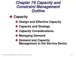
2. Outline • Capacity • Design and Effective Capacity • Capacity and Strategy • Capacity Considerations • Managing Demand • Demand and Capacity Management in the Service Sector • Bottleneck Analysis and Theory of Constraints • Process Times for Stations, Systems, and Cycles • Break-Even Analysis

3. Learning Objectives When you complete this supplement, you should be able to: Define capacity Determine design capacity, effective capacity, and utilization Perform bottleneck analysis Compute break-even analysis

4. Capacity • The throughput, or the number of units a facility can hold, receive, store, or produce in a period of time • Determines fixed costs • Determines if demand will be satisfied • Three time horizons

5. Options for Adjusting Capacity * Long-range planning Add facilities Add long lead time equipment Intermediate-range planning Subcontract Add personnel Add equipment Build or use inventory Add shifts Schedule jobs Schedule personnel Allocate machinery * Short-range planning Modify capacity Use capacity * Difficult to adjust capacity as limited options exist Planning Over a Time Horizon Figure S7.1

6. Design and Effective Capacity • Design capacity is the maximum theoretical output of a system • Normally expressed as a rate • Effective capacity is the capacity a firm expects to achieve given current operating constraints • Often lower than design capacity

7. Utilization and Efficiency Utilization is the percent of design capacity achieved Utilization = Actual output/Design capacity Efficiency is the percent of effective capacity achieved Efficiency = Actual output/Effective capacity

8. Bakery Example Actual production last week = 148,000 rolls Effective capacity = 175,000 rolls Design capacity = 1,200 rolls per hour Bakery operates 7 days/week, 3 - 8 hour shifts Design capacity = (7 x 3 x 8) x (1,200) = 201,600 rolls

9. Bakery Example Actual production last week = 148,000 rolls Effective capacity = 175,000 rolls Design capacity = 1,200 rolls per hour Bakery operates 7 days/week, 3 - 8 hour shifts Design capacity = (7 x 3 x 8) x (1,200) = 201,600 rolls

10. Bakery Example Actual production last week = 148,000 rolls Effective capacity = 175,000 rolls Design capacity = 1,200 rolls per hour Bakery operates 7 days/week, 3 - 8 hour shifts Design capacity = (7 x 3 x 8) x (1,200) = 201,600 rolls Utilization = 148,000/201,600 = 73.4%

11. Bakery Example Actual production last week = 148,000 rolls Effective capacity = 175,000 rolls Design capacity = 1,200 rolls per hour Bakery operates 7 days/week, 3 - 8 hour shifts Design capacity = (7 x 3 x 8) x (1,200) = 201,600 rolls Utilization = 148,000/201,600 = 73.4%

12. Bakery Example Actual production last week = 148,000 rolls Effective capacity = 175,000 rolls Design capacity = 1,200 rolls per hour Bakery operates 7 days/week, 3 - 8 hour shifts Design capacity = (7 x 3 x 8) x (1,200) = 201,600 rolls Utilization = 148,000/201,600 = 73.4% Efficiency = 148,000/175,000 = 84.6%

13. Bakery Example Actual production last week = 148,000 rolls Effective capacity = 175,000 rolls Design capacity = 1,200 rolls per hour Bakery operates 7 days/week, 3 - 8 hour shifts Design capacity = (7 x 3 x 8) x (1,200) = 201,600 rolls Utilization = 148,000/201,600 = 73.4% Efficiency = 148,000/175,000 = 84.6%

14. Bakery Example Actual production last week = 148,000 rolls Effective capacity = 175,000 rolls Design capacity = 1,200 rolls per hour Bakery operates 7 days/week, 3 - 8 hour shifts Efficiency = 84.6% Efficiency of new line = 75% Expected Output = (Effective Capacity)(Efficiency) = (175,000)(.75) = 131,250 rolls

15. Bakery Example Actual production last week = 148,000 rolls Effective capacity = 175,000 rolls Design capacity = 1,200 rolls per hour Bakery operates 7 days/week, 3 - 8 hour shifts Efficiency = 84.6% Efficiency of new line = 75% Expected Output = (Effective Capacity)(Efficiency) = (175,000)(.75) = 131,250 rolls

16. Managing Demand • Demand exceeds capacity • Curtail demand by raising prices, scheduling longer lead time • Long term solution is to increase capacity • Capacity exceeds demand • Stimulate market • Product changes • Adjusting to seasonal demands • Produce products with complementary demand patterns

17. Combining both demand patterns reduces the variation 4,000 – 3,000 – 2,000 – 1,000 – Snowmobile motor sales Sales in units Jet ski engine sales J F M A M J J A S O N D J F M A M J J A S O N D J Time (months) Complementary Demand Patterns Figure S7.3

18. Demand and Capacity Management in the Service Sector • Demand management • Appointment, reservations, FCFS rule • Capacity management • Full time, temporary, part-time staff

19. Break-Even Analysis • Objective is to find the point in dollars and units at which cost equals revenue • Fixed costs are costs that continue even if no units are produced • Depreciation, taxes, debt, mortgage payments • Variable costs are costs that vary with the volume of units produced • Labor, materials, portion of utilities • Assumes - Costs and revenue are linear

20. – 900 – 800 – 700 – 600 – 500 – 400 – 300 – 200 – 100 – – Total revenue line Total cost line Break-even point Total cost = Total revenue Profit corridor Cost in dollars Variable cost Loss corridor Fixed cost | | | | | | | | | | | | 0 100 200 300 400 500 600 700 800 900 1000 1100 Volume (units per period) Break-Even Analysis Figure S7.5

21. BEPx = break-even point in units BEP$ = break-even point in dollars P = price per unit (after all discounts) x = number of units produced TR = total revenue = Px F = fixed costs V = variable cost per unit TC = total costs = F + Vx F P - V BEPx = Break-Even Analysis Break-even point occurs when TR = TC or Px = F + Vx

22. BEPx = break-even point in units BEP$ = break-even point in dollars P = price per unit (after all discounts) x = number of units produced TR = total revenue = Px F = fixed costs V = variable cost per unit TC = total costs = F + Vx BEP$ = BEPxP = P = = F P - V F 1 - V/P F (P - V)/P Break-Even Analysis Profit = TR - TC = Px - (F + Vx) = Px - F - Vx = (P - V)x - F

23. BEP$ = = F 1 - (V/P) $10,000 1 - [(1.50 + .75)/(4.00)] Break-Even Example Fixed costs = $10,000 Material = $.75/unit Direct labor = $1.50/unit Selling price = $4.00 per unit

24. BEP$ = = F 1 - (V/P) = = $22,857.14 BEPx = = = 5,714 $10,000 1 - [(1.50 + .75)/(4.00)] $10,000 .4375 $10,000 4.00 - (1.50 + .75) F P - V Break-Even Example Fixed costs = $10,000 Material = $.75/unit Direct labor = $1.50/unit Selling price = $4.00 per unit

25. 50,000 – 40,000 – 30,000 – 20,000 – 10,000 – – Revenue Break-even point Total costs Dollars Fixed costs | | | | | | 0 2,000 4,000 6,000 8,000 10,000 Units Break-Even Example

26. F BEP$= ∑1 - x (Wi) Vi Pi Break-Even Example Multiproduct Case where V = variable cost per unit P = price per unit F = fixed costs W = percent each product is of total dollar sales i = each product

27. In-Class Problems from the Lecture Guide Practice Problems Problem 1: The design capacity for engine repair in our company is 80 trucks/day. The effective capacity is 40 engines/day and the actual output is 36 engines/day. Calculate the utilization and efficiency of the operation. If the efficiency for next month is expected to be 82%, what is the expected output?

28. In-Class Problems from the Lecture Guide Practice Problems Problem 5: Jack’s Grocery is manufacturing a “store brand” item that has a variable cost of $0.75 per unit and a selling price of $1.25 per unit. Fixed costs are $12,000. Current volume is 50,000 units. The Grocery can substantially improve the product quality by adding a new piece of equipment at an additional fixed cost of $5,000. Variable cost would increase to $1.00, but their volume should increase to 70,000 units due to the higher quality product. Should the company buy the new equipment?

29. In-Class Problems from the Lecture Guide Practice Problems Problem 6: What are the break-even points ($ and units) for the two processes considered in Problem S7.5?

30. In-Class Problems from the Lecture Guide Practice Problems Problem 7: Develop a break-even chart for Problem S7.5.