Download
1 / 10
120 likes | 276 Views
Multiple Linear Regression. For k>1 number of explanatory variables. e.g.: Exam grades as function of time devoted to study, as well as SAT scores.

E N D
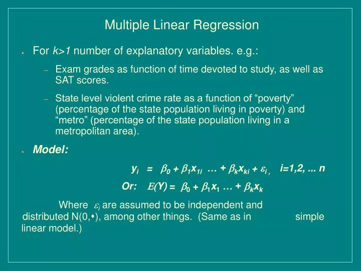
Multiple Linear Regression For k>1 number of explanatory variables. e.g.: Exam grades as function of time devoted to study, as well as SAT scores. State level violent crime rate as a function of “poverty” (percentage of the state population living in poverty) and “metro” (percentage of the state population living in a metropolitan area). Model: yi = 0 + 1x1i … + kxki + i , i=1,2, ... n Or: E(Y) = 0 + 1x1 … + kxk Where i are assumed to be independent and distributed N(0,s), among other things. (Same as in simple linear model.)
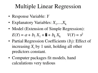
Multiple Linear Regression Meaning of k: A one unit increase in xk is associated with k units increase in E(y), holding all other x's constant. If k is 0 in the population, then there is no relationship between xk and y (for any i). k is called the “marginal effect” of xk on E(y). Meaning of 0: E(y) when all x=0. How to find the “best” 's? According to the same OLS principle Now fitting a “plane” in k+1 dimensional space, rather than a line in 2 dimensional space. (Imagine k=2 case.) We minimize the sum of squared errors from observed data points to the regression plane. Property of OLS estimators (under the “classical linear model assumptions”): BLUE (best linear unbiased estimator).
Multiple Linear Regression ExampleViolent Crime Rates = f(poverty, metro) • The estimated regression model is • E(Crime) = -636.54 + 41.31*Poverty + 9.43*Metro • Mean(Poverty)=13.01%, mean(Metro)=67.89. • For all states with Poverty=13.01% and Metro= 67.89%, we predict the average violent crime rate to be -636.54 + 41.31*13.01 + 9.43*67.89 = 541 (per 100,000 population) • Prediction for an individual state is the same, but with higher uncertainty due to the random error term. • The marginal effect of “poverty” on the average crime rate, holding “metro” constant (at any value), is 41.31---every 1% increase in“poverty” corresponds to 41.31 more cases of violent crime per 100k population.
The estimated k values are based on one particular sample set, and so are the sample intercept/slopes. What are the corresponding population parameters? Testing a population slope (intercept similar, but less interesting) being zero (i.e., testing the hypothesis that there is no relationship between some x and y): Recall logic of hypothesis test Under the null hypothesis, the sampling distribution of the estimated k/sd(k) is shown to follow the “Student-t” distribution (assuming s unknown) with n-k-1 degrees of freedom Software routinely reports the p-values from the test We can also test the “global” hypothesis that all k's are simultaneously 0, i.e., our independent variables as a group have no significant effect on our dependent variable. “F-test”, p-values for F(1,n-k-1) routinely reported by software. Rejecting null means: at least one x “matters”. Hypothesis Testing: Is There a Relationship?
Goodness of Fit: the Coefficient of Determination (R2) Measures how well the regression model fits the data R2 measures how much variation in the values of the response variable (y) is explained by the regression model (i.e., by all the independent variables collectively) The distance between an observed Y and the mean of Y in the data set can be decomposed into two parts: from Y to E(Y) given by the regression model, and from E(Y) to the mean of all Y. R2is define as RSS/TSS. The higher the R2, the better the fit. Adding more independent variables to the model never decreases R2---some software reports the “adjusted R2“to account for model complexity. (Ultimately, goodness of fit measures should not be used as the model selection criterion, as a model could possibly over-fit the data. Compare out-of-sample prediction performance instead.)
OLS not robust to outliers (regardless of the number of x variables) Extrapolation beyond observed data region dangerous Correlation does not imply causation Properties of OLS estimators hold only if the model assumptions are satisfied Beware...
Stata example: sysuse lifeexp; reg lexp safewater gnppc Using Software
Dummy X Variables • Sometimes one or more of our independent variables may be categorical variables, such as gender or race. • Multiple valued categorical variables can be recoded into a set of binary “dummy” variables taking values 0/1. e.g. White/Black/Hispanic/Asian (Why we don't want to use the multiple valued variable “race” in the regression model, if it's coded say 1,2,3,4?) • If there are m categories, we use m-1 dummies in the model, since the last one does not add any information: knowing the value of “White”, “Black”, and “Hispanic” we can infer the value of “Asian” (assuming these exhaust the racial categories in the data). Similarly, for “gender” we only need one variable, not two.
Dummy X Variables • If xk is a dummy variable in the model E(Y)=0+1x1 …+kxk, then k measures the change in E(Y) associated with xk going from 0 to 1, or the difference between the intercepts for the two categories (e.g., male/female) • For multiple dummies recoded from multiple valued categorical variables such as “race”, the coefficient of each dummy reflects the difference between the corresponding category and the “base” category left out of the model. • e.g. If using “White”, “Black”, and “Hispanic” in the model, then the coefficient of “White” measures the difference in the intercept between “White” and “Asian”. • Stata eg. Sysuse nlsw88; tabulate race,generate(race1) • reg wage race11 race12 tenure union south • gen racesouth=race12*south • reg wage race11 race12 tenure union south racesouth
Interaction Effects: Special Case of Non-Linearity • In the additive model, the marginal effect of some x on E(y) is constant, independent of the values of the other x's in the model. This is generally not true in a non-linear model. • Interaction effect model is a special case of a non-linear model. Simple example: E(Y) = 0 + 1x1 + 2x2 +3x1x2 • In this model, the marginal effect of x1 depends on the value of x2. • e.g. X1 = Gender (female=1), x2 = Education (high=1), Y=Pro-choice abortion opinion (higher score-->stronger pro-choice views) • Estimated model: (showing reversed gender gap for low educ) • E(Y) = 4.04 - .55x1 + 1.09 x2 + 1.16 x1 x2 • male/low educ: 4.04; • female/low educ: 4.04-.55; • male/high educ: 4.04+1.09; • female/high educ: 4.04-.55+1.09+1.16