Download

1 / 39
430 likes | 758 Views
MECH 221 FLUID MECHANICS (Fall 06/07) Chapter 3: FLUID IN MOTIONS. Instructor: Professor C. T. HSU. 3.1. Newton’s Second Law. The net force F acting on a matter of mass m leads to an acceleration a following the linear relation: F = m a

E N D
MECH 221 FLUID MECHANICS(Fall 06/07)Chapter 3: FLUID IN MOTIONS Instructor: Professor C. T. HSU
3.1. Newton’s Second Law • The net force F acting on a matter of mass m leads to an acceleration a following the linear relation: F= ma • For a solid body of fixed shape, m is a constant and a is described along the trajectory of motion.
3.1. Newton’s Second Law • If r(t) represents the particle trajectory, the velocity v(t) and acceleration are then given by: v(t) = dr/dt ; a(t) = dv/dt = d2r/dt2 • Therefore, F= mdv/dt • If m = m(t), then F = (mdv/dt)+(vdm/dt)=d(mv)/dt = dM/dt. where M = mv is the momentum.
3.1. Newton’s Second Law • For fluids enclosed in a control volume V(t) which may deform with time along the trajectory of motion, it is only correct to use the fluid momentum M to describe the Newton’s second law • For M= , we have F = dM/dt =
3.2. Description of Fluid Flow • Fluid dynamics is the mechanics to study the evolution of fluid particles in a space domain (flow field). There are two ways to describe the flow field • Lagrangian description • Eulerian description
3.2.1 Lagrangian Description • Given initially the locations of all the fluid particles, a Lagrangian description is to follow historically each particle motion by finding the particle locations and properties at every time instant.
3.2.1 Lagrangian Description • Therefore, if a specific fluid particle is initially (t=t0) located at (x0, y0, z0), the Lagragian description is to determine (x(t), y(t), z(t)) and the fluid properties, such as f(t) = f [x(t), y(t), z(t); t], v(t) = v [x(t), y(t), z(t); t] , etc. given f0 = f (x0, y0, z0; t0), v0 = v (x0, y0, z0; t0) etc. • Note that (x(t), y(t), z(t)) is a function of time. (for any function f)
3.2.2. Eulerian Description • An Eulerian description of fluid flow is simply to state the evolution of fluid properties at a fixed point (x, y, z) with time. Here (x, y, z) is independent of time. Hence, f(t) = f[x, y, z, t] , v = v [x, y ,z, t] etc. • Eulerian description is to observe the fluid properties of different fluid particles passing through the same fixed location at different time instant, while Lagrangian description is to observe the fluid properties at different locations following the same particle
3.2.3. Relation between Lagrangian and Eulerian description • It is important to note that there is only one flow property at the same location with respect to the same time, i.e., f(x(t),y(t),z(t),t) = f(x,y,z,t). Therefore, the Lagrange differential with respective to dt, which is equal to the total Eulerian differential:
3.2.3. Relation between Lagrangian and Eulerian description • Hence, the total derivative is given by:
3.3. Equations of Motion for Inviscid Flow • Conservation of Mass • Conservation of Momentum
3.3.1. Conservation of Mass • Mass in fluid flows must conserve. The total mass in V(t) is given by: • Therefore, the conservation of mass requires that dm/dt = 0. where the Leibniz rule was invoked.
3.3.1. Conservation of Mass • Hence: This is the Integral Form of mass conservation equation.
= 0 3.3.1. Conservation of Mass • Integral form of mass conservation equation • By Divergence theorem: • Hence:
3.3.1. Conservation of Mass • As V(t)→0, the integrand is independent of V(t) and therefore, This is the Differential Form of mass conservation and also called as continuity equation.
3.3.2. Conservation of Momentum • The Newton’s second law, is Lagrangian in a description of momentum conservation. For motion of fluid particles that have no rotation, the flow is termed irrotational. An irrotational flow does not subject to shear force, i.e., pressure force only. Because the shear force is only caused by fluid viscosity, the irrotational flow is also called as “inviscid” flow
3.3.2. Conservation of Momentum • For fluid subjecting to earth gravitational acceleration, the net force on fluids in the control volume V enclosed by a control surface S is: where s is out-normal to S from V and the divergence theorem is applied for the second equality. • This force applied on the fluid body will leads to the acceleration which is described as the rate of change in momentum.
3.3.2. Conservation of Momentum where the Leibniz rule was invoked.
3.3.2. Conservation of Momentum • Hence: This is the Integral Form of momentum conservation equation.
3.3.2. Conservation of Momentum • Integral form of momentum conservation equation • By Divergence theorem: • Hence:
3.3.2. Conservation of Momentum • As V→0, the integrands are independent of V. Therefore, This is the Differential Form of momentum conservation equation for inviscid flows.
3.3.2. Conservation of Momentum • By invoking the continuity equation, • The momentum equation can take the following alternative form: which is commonly referred to as Euler’s equation of motion.
3.4. Bernoulli Equation for Steady Flows • Bernoulli equation is a special form of the Euler’s equation along a streamline. For a first look, we restrict our discussion to steady flow so that the Euler’s equation becomes: • Assuming that g is in the negative z direction, i.e., g =- and using the following vector identity, the Euler’s equation for steady flows becomes
(for any function f) ; 3.4. Bernoulli Equation for Steady Flows • We now take the scalar product to the above equation by the position increment vector dralong a streamline and observe that • Thus, the result leads to • The above equation now can be integrated to give (along streamline)
3.4. Bernoulli Equation for Steady Flows • For incompressible fluids where ρ = constant, we have • For irrotational flows, everywhere in the flow domain and (along streamline)
3.4. Bernoulli Equation for Steady Flows • Since, for dr in any direction, we have: • For anywhere of irrotational fluids • For anywhere of incompressible fluids
3.5. Static, Dynamic, Stagnation and Total Pressure • Consider the Bernoulli equation, • The static pressure ps is defined as the pressure associated with the gravitational force when the fluid is not in motion. If the atmospheric pressure is used as the reference for a gage pressure at z=0. (for incompressible fluid)
3.5. Static, Dynamic, Stagnation and Total Pressure • Then we have as also from chapter 2. • The dynamic pressure pd is then the pressure deviates from the static pressure, i.e., p = pd+ps. The substitution of p = pd+ps. into the Bernoulli equation gives
3.5. Static, Dynamic, Stagnation and Total Pressure • The maximum dynamic pressure occurs at the stagnation point where v=0 and this maximum pressure is called as the stagnation pressure p0. Hence, • The total pressure pT is then the sum of the stagnation pressure and the static pressure, i.e., pT= p0 - ρgz. For z = -h, the static pressure is ρgh and the total pressure is p0 + ρgh.
3.6. Energy Line and Hydraulic Grade Line • In fact the Bernoulli equation also states that the energy density (per unit volume) possessed by the fluid particle is constant not only along a streamline but also at everywhere in fluid domain for irrotational flow. The energy consists of pressure energy (p), kinetic energy (ρv2/2) and gravitational potential energy (ρgz).
3.6. Energy Line and Hydraulic Grade Line • It becomes simpler if this total energy is interpreted into a total head H (height from a datum) by dividing the Bernoulli equation with ρg such that where p/ρg is the pressure head, v2/2g is the velocity head and z is the elevation head.
3.6. Energy Line and Hydraulic Grade Line • A piezometric head is then defined as that consists of only the pressure and elevation heads, i.e., • The variations of H and Hp along the path of fluid flow can be plotted into lines and are termed as “energy line” and “hydraulic grade line”, respectively. • It is noted that H is always higher than Hp and that a negative pressure (below atmospheric pressure) occurs when Hp is below the fluid streamline
3.7. Applications of Bernoulli Equation • Pitot-Static Tube • Free Jets • Flow Rate Meter
3.7.1. Pitot-Static Tube • Pitot-static tube is a device that measures the difference between h1 and h2 so that the velocity of the fluid flow at the measurement location can be determined from
3.7.2. Free Jets • Free jets are the flow from an orifice of an apparatus that converts the total elevation head h into velocity head, i.e.,
3.7.3. Flow Rate Meter • The commonly used flow rate meter is the Venturi meter that determines the flow rate Q through pipes by measuring the difference of piezometric heads at locations of different cross-sectional areas along the pipe.
and Then, Therefore, 3.7.3. Flow Rate Meter • If hp1 and hp2 represent the piezometric heads at section 1 and 2 with cross-sectional areas A1 and A2 respectively, we have: