Download
1 / 1
10 likes | 126 Views
Diagnosis of the Ozone Budget in the SH Lower Stratosphere Wuhu Feng and Martyn Chipperfield School of the Environment, University of Leeds, Leeds, UK, LS2 9JT Howard Roscoe British Antarctic Survey, Cambridge, UK. 4. Results: Comparison with APE Data. 1. Introduction

E N D
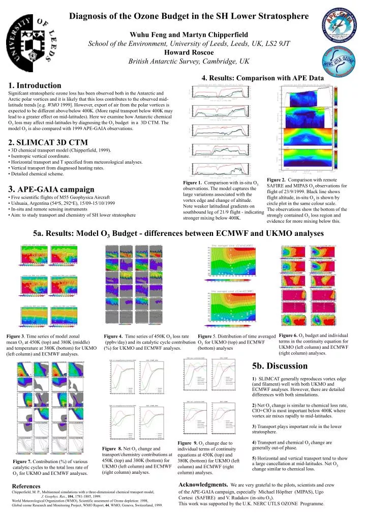
Diagnosis of the Ozone Budget in the SH Lower Stratosphere Wuhu Feng and Martyn Chipperfield School of the Environment, University of Leeds, Leeds, UK, LS2 9JT Howard Roscoe British Antarctic Survey, Cambridge, UK 4. Results:Comparison with APE Data 1. Introduction Signifcant stratospheric ozone loss has been observed both in the Antarctic and Arctic polar vortices and it is likely that this loss contributes to the observed mid-latitude trends [e.g. WMO 1999]. However, export of air from the polar vortices is expected to be different above/below 400K. (More rapid transport below 400K may lead to a greater effect on mid-latitudes). Here we examine how Antarctic chemical O3 loss may affect mid-latitudes by diagnosing the O3 budget in a 3D CTM. The model O3 is also compared with 1999 APE-GAIA observations. 2. SLIMCAT 3D CTM • 3D chemical transport model (Chipperfield, 1999). • Isentropic vertical coordinate. • Horizontal transport and T specified from meteorological analyses. • Vertical transport from diagnosed heating rates. • Detailed chemical scheme. Figure 2. Comparison with remote SAFIRE and MIPAS O3 observations for flight of 23/9/1999. Black line shows flight altitude, in-situ O3 is shown by circle plot in the same colour scale. The observations show the bottom of the strongly contained O3 loss region and evidence for more mixing below this. Figure 1. Comparison with in-situ O3 observations. The model captures the large variations associated with the vortex edge and change of altitude. Note weaker latitudinal gradients on southbound leg of 21/9 flight - indicating stronger mixing below 400K. 3. APE-GAIA campaign • Five scientific flights of M55 Geophysica Aircraft • Ushuaia, Argentina (54oS, 292oE), 15/09-15/10/1999 • In-situ and remote sensing instruments • Aim: to study transport and chemistry of SH lower stratosphere 5a. Results: Model O3 Budget - differences between ECMWF and UKMO analyses Figure 6. O3 budget and individual terms in the continuity equation for UKMO (left column) and ECMWF (right column) analyses. Figure 3. Time series of model zonal mean O3 at 450K (top) and 380K (middle) and temperature at 380K (bottom) for UKMO (left column) and ECMWF analyses. Figure 4. Time series of 450K O3 loss rate (ppbv/day) and its catalytic cycle contribution (%) for UKMO and ECMWF analyses. Figure 5. Distribution of time averaged O3 for UKMO (top) and ECMWF (bottom) analyses 5b. Discussion 1) SLIMCAT generally reproduces vortex edge (and filament) well with both UKMO and ECMWF analyses. However, there are detailed differences with both simulations. 2) Net O3 change is similar to chemical loss rate, ClO+ClO is most important below 400K where vortex air mixes rapidly to mid-latitudes. 3) Transport plays important role in the lower stratosphere. 4) Transport and chemical O3 change are generally out-of phase. 5) Horizontal and vertical transport tend to show a large cancellation at mid-latitudes. Net O3 change similar to chemical loss. Figure 9. O3 change due to individual terms of continuity equations at 450K (top) and 380K (bottom) for UKMO (left column) and ECMWF (right column) analyses. Figure 8. Net O3 change and transport/chemistry contributions at 450K (top) and 380K (bottom) for UKMO (left column) and ECMWF (right column) analyses. Figure 7.Contribution (%) of various catalytic cycles to the total loss rate of O3 for UKMO and ECMWF analyses. Acknowledgments.We are very grateful to the pilots, scientists and crew of the APE-GAIA campaign, especially Michael Höpfner (MIPAS), Ugo Cortesi (SAFIRE) and V. Rudakov (in-situ O3). This work was supported by the U.K. NERC UTLS OZONE Programme. References Chipperfield, M. P., Multiannual simulations with a three-dimensional chemical transport model, J. Geophys. Res., 104, 1781-1805, 1999. World Meteorological Organization (WMO), Scientific assesment of Ozone depletion: 1998, Global ozone Research and Monitoring Project, WMO Report, 44, WMO, Geneva, Switzerland, 1999.