Download
1 / 38
380 likes | 548 Views
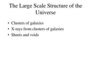
Supernovae and scale of the universe. SN Ia have extremely uniform light curves → standard candles!. Supernovae and scale of the universe.

E N D
SN Ia have extremely uniform light curves → standard candles!
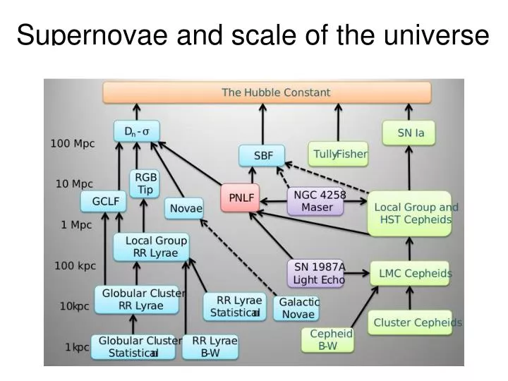
Supernovae and scale of the universe The cosmic distance ladder (also known as the Extragalactic Distance Scale) is the succession of methods by which astronomers determine the distances to celestial objects. A real direct distance measurement to an astronomical object is only possible for those objects that are "close enough" (within about a thousand parsecs) to Earth. The techniques for determining distances to more distant objects are all based on various measured correlations between methods that work at close distances with methods that work at larger distances. Several methods rely on a standard candle, which is an astronomical object that has a known luminosity. Type Ia supernovae that have a very well-determined maximum absolute magnitude as a function of the shape of their light curve and are useful in determining extragalactic distances up to a few hundred Mpc
Hubble’s “Law” Hubble showed that galaxies recede from us in all directions and more distant ones recede more rapidly in proportion to their distance. His graph of velocity against distance is the original Hubble diagram; the equation that describes the linear fit, velocity = Ho × distance, is Hubble's Law; the slope of that line is the Hubble constant, Ho; and 1/Ho is the Hubble time. next few slides are from http://www.pnas.org/content/101/1/8.full
Published values of the Hubble constant vs. time. Revisions in Hubble's original distance scale account for significant changes in the Hubble constant from 1920 to the present as compiled by John Huchra of the Harvard–Smithsonian Center for Astrophysics. At each epoch, the estimated error in the Hubble constant is small compared with the subsequent changes in its value. This result is a symptom of underestimated systematic errors.
The Hubble diagram for type Ia supernovae. From the compilation of well observed type Ia supernovae by Jha (29). The scatter about the line corresponds to statistical distance errors of <10% per object. The small red region in the lower left marks the span of Hubble's original Hubble diagram from 1929.
Hubble diagram for type Ia supernovae to z ≈ 1. Plot in astronomers' conventional coordinates of distance modulus (a logarithmic measure of the distance) vs. log redshift. The history of cosmic expansion can be inferred from the shape of this diagram when it is extended to high redshift and correspondingly large distances.
Deviations in the Hubble Diagram • The difference at each redshift between the measured apparent brightness and the expected location in the Hubble diagram in a universe that is expanding without any acceleration or deceleration. The blue points are median values in eight redshift bins. • The upward bulge at z ≈ 0.5 is the signature of cosmic acceleration. • From top to bottom, the plotted lines correspond to: • the favored solution, with 30% dark matter and 70% dark energy • the observed amount of dark matter (30%) but no dark energy; • a universe with 100% dark matter
Hubble Space Telescope images show supernovae (arrows) in three distant galaxies. [P. Garnavich (CfA)/High-z Supernova Search Team/NASA]
Initially the universe was a dense, hot cauldron of particles of matter and energy. • Disturbances in this dense soup set off sound ripples. These sound waves helped matter begin to clump together, forming the first structure in the universe. We see the result of this clumping in the cosmic microwave background radiation. • The ripples also established a basic "yardstick" for the distribution of matter. As the universe expands, the yardstick expands with it. By measuring the size of the yardstick at different times in the history of the universe, astronomers can plot how the rate of expansion of the universe has changed. • The yardstick was preserved as the universe expanded but it’s not easy to detect. A look at even a tiny region of the sky reveals millions of galaxies distributed through space and time — some of them are quite close while others are billions of light-years away. • So astronomers must measure millions of galaxies, isolate them by distance (which means at different ages of the universe), then analyze the patterns at different epochs. • HETDEX will produce a 3-D map of at least one million galaxies that are roughly 9 billion to 11 billion light-years away.
HETDEX will map galaxies at different times in the history of the universe to try to find the "imprint" of sound waves from the very early universe. • Left: A field of galaxies for study. • Center: Astronomers will measure the distances between millions of galaxy pairs, and use statistics to find a common "scale length." • Right: This common length is the imprint of the early sound waves, which shows up as "ripples" in the distribution of galaxies. • The scale length changes as the universe ages, so determining that length at different epochs will reveal how the expansion rate of the universe has changed over time.
Distribution of galaxies in the universe Large scale structure inferred from galaxy redshifts. Each dot in this plot marks a galaxy whose distance is estimated from its redshift by using Hubble's Law. From the 2DF Galaxy Redshift Survey
Four images of the fiber bundles that carry light to the VIRUS spectrograph.
Ancillary science? • Astronomers expect that during any single observation, fewer than one percent of the fibers will be pointing at galaxies. • Even so, the experiment will take data on several hundred galaxies during each observation, which will last around 20 minutes. • After an observation is completed, the telescope will be moved slightly to view the next patch of sky, providing several dozen observations per night. • HETDEX will conduct about 140 nights of observing, providing spectra for at least one million galaxies. • AND! What else?
Ordinary metal-poor giant - simulation Mediocre high res Sloan-ish HETDEX/VIRUS
Beers et al. 1985 R ~ 2000 observations and models
HK Survey discovery spectra Beers, Preston, & Shectman 1985, AJ, 90, 2089 Bandpass: 3875-4025Å R = λ/Δλ ~ 900
This is what we will see CH H&K H H
Better than the original HK survey by far • Fainter by several mags • Flux information • Higher S/N • Balmer line information • C-rich low metallicity “easy” detection Who needs Sloan?