Download
1 / 22
220 likes | 566 Views
Estimating Seed and Invertebrate Production to Predict Waterfowl Carrying Capacity in Moist-soil Habitats Matthew J. Gray James T. Anderson, Richard M. Kaminski, and Loren M. Smith What is Carrying Capacity?

E N D
Estimating Seed and Invertebrate Production to Predict Waterfowl Carrying Capacity in Moist-soil Habitats Matthew J. Gray James T. Anderson, Richard M. Kaminski, and Loren M. Smith
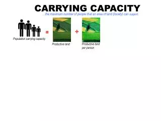
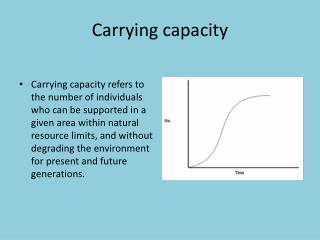
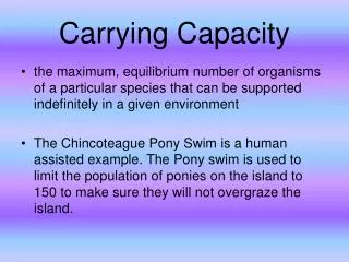
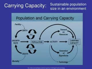
What is Carrying Capacity? “Maximum number of individuals that can be ‘sustained’ in a given ‘habitat’ for a ‘given amount of time’.” (Krebs 1993) “There is a maximum wild density of individuals that can be supported in the environment” (Leopold 1931, Stoddard 1931,Leopold 1933) “…the heaviest quail/muskrat population that can be expected to survive winter,” is dependent on the “…availability of suitable food and cover...” (Errington 1934, 1936, 1945, 1947)
“The amount of food for each species…gives the extreme limit to which ‘a population’ can increase…” (Darwin 1909, The Origin of Species) Carrying Capacity of Food Resources “… carrying capacity of food ‘resources’ …” (Leopold 1933) “… the quantity of food necessary to feed 1 duck for 1 day… ” is equivalent to 1 duck use-day. (Prince 1979, Reinecke et al. 1989)
Quantifying Waterfowl Use-Days Prince 1979 Reinecke et al. 1989 Reinecke and Loesch 1996 Food Available (g [dry]) x MTE (kcal/g [dry]) WUD = Daily Energy Requirement (kcal/day) Available Food for Waterfowl MTE Constants DER Constant Moist-soil Seeds 2.5 kcal/g 292 kcal/day Aquatic Invertebrates 3.5 kcal/g
Why Estimate Waterfowl Use-days? To Predict Wetland-Specific Waterfowl Carrying Capacity • To Evaluate Management Practices
Collecting Sorting Estimating Seed and Invertebrate Production Seeds Invertebrates Clipping Field Work Threshing Lab Work Specialized Equipment Nets, Clippers, Refrigerated Storage, Sieves, Sorting Trays, Dryer, Desiccator, Balance
Estimating Seed Yield of Moist-soil Plants using Multiple Linear Regression Yi = ß0 + ß1 X1i + ß2 X2i + ••• + ßk Xki +εi Dependent Variable (Laubhan and Fredrickson 1992) Y IL Seed Yield (g) IL Predictor Variables ID ID Phyto-morphological Measurements (cm)
1) Plant morphology can vary spatially and temporally Yi = ßk Xki +εi Research Justification 2) Measuring multiple floristic variables can be tedious and confusing 3) Equations for aquatic invertebrates have not been developed
1) Evaluate Laubhan and Fredrickson’s method in a different location and in different years Research Objectives 2) Evaluate different phyto-morphological measurements as predictor variables 3) Develop a new method to predict seed yield of moist-soil plants with a single, easily measured variable 4) Develop new regression equations to predict aquatic invertebrate biomass
Prisock Moist-soil Management Complex Study Areas and Years (1993, 1994) Mississippi Noxubee National Wildlife Refuge Southern High Plains 12 Playa Lakes Floyd County Texas (1994, 1995)
Flower Width & Length Pedicel Methods:Plant Morphological Study 5 species::Echinochloa crusgalli, Cyperus erythrorhizos, Polygonum hydropiperoides, Panicum dichotomiflorum, Rynchospora globularis n = 60 plants/species/year, 1993 and 1994 L & F (1992) New Variables • Plant Height • Inflorescence Length • Infl. Base Diameter • Infl. Volume • # of Inflorescences • Number of Pedicels • Number of Flowers • Flower Width • Flower Height Seed Processing followed L&F (1992)
Methods:Dot Study 5 species::Echinochloa crusgalli, Setaria viridis, Panicum agrostoides, Panicum dichotomiflorum, Rynchospora globularis n = 30 plants/species/year, 1994 Preparation Processing • Plant Press • 7 days • Room Temperature • Pedicels Separated • Dot grid (9 dots/cm2) • Dots Obscured by Seed Counted Seed Processing followed L&F (1992)
Methods:Aquatic Invertebrate Study Invertebrate Collection and Processing Water-Column (5-cm diameter) Epiphytic Sample (0.25-m2 plot) Benthic Core (5-cm diameter) • 20 subsamples/playa • 2 sampling episodes/week • September-January • Sorted and identified • Dried to constant mass • g dry inverts/playa/week/m2
Methods:Aquatic Invertebrate Study Predictor Variables Water Variables: • Conductivity • Dissolved Oxygen • Temperature • pH • Water Depth Induced Variables: • Inundation duration • Treatment (managed, unmanaged)
Statistical Analysis Simple and Multiple Linear Regression Assumptions: • Residual Normality • Residual Homoscedasticity Residual Plots & Outlier Diagnostics Model Development: All-possible Variable Selection Procedure • Greatest R2adjusted • Lowest MSE • Mallow’s Cp p • Greatest R2predicted (PRESS) Multicollinearity: VIF > 10, EV 0, CN > 10
OKAY!!! HERE’S THE GOOD STUFF!! Results and Discussion
Our Data L & F Best Model L & F (1992) Dot Model R2adjusted Seed Prediction Results: 4 Models 0.68-0.920.78-0.970.79-0.96 0.92-0.97 R2predicted 0.23-0.880.31-0.97NAV 0.91-0.96 MSE 0.002-0.39 0.001-0.18 NAV 0.001-0.009 Cp 48.2-495.0 3.9-6.6 NAV NAP VIF 1.1-34.83.9-12.0 NAV NAP NAV= Not Available,NAP = Not Applicable
Invertebrate Prediction Results (Single Variable Models) R2adjusted R2predicted MSE • Increasing p,Increased R2< 0.03 • Increasing p,Increased VIF > 10 Conductivity 0.6040.582 333.14 Treatment 0.5870.562 347.48 pH 0.5810.564 352.83 DO 0.4940.483 426.40 Depth 0.4690.451 449.09 Time 0.3960.379 508.49 Temperature 0.3710.365 529.34
Summary of Results Simple linear regression models can explain as much variation in seed yield and aquatic invertbrate biomass and predict as well or better than multiple regression models. Seed (g) = 0.003 x DOTS Seed Yield/ Invert Biomass Inverts (g) = 0.023 x COND Dots Obscured/Conductivity
(Single-variable Models) Management Applicability Easy Fast Reasonable Cost • Plant Press ($35) • Dot Grid ($10) • Conductivity/pH Meter ($50-350)
Future Research Needs Additional Models Spatial Replication Systems, Regions Temporal Replication
Waterways Experiment Station (Wetland Research Program) Funding Agencies U.S. Fish & Wildlife Service Regions 2 and 4 U.S. Geological Survey U.S. Army Corps of Engineers Biological Resources Division Texas Tech University Mississippi State University Department of Range, Wildlife, and Fisheries Department of Wildlife and Fisheries