Download
1 / 55
550 likes | 553 Views
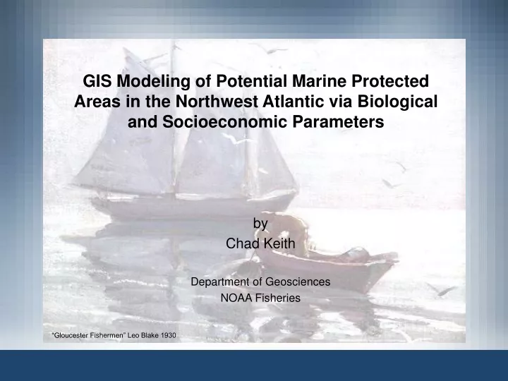
GIS Modeling of Potential Marine Protected Areas in the Northwest Atlantic via Biological and Socioeconomic Parameters. by Chad Keith Department of Geosciences NOAA Fisheries. “Gloucester Fishermen” Leo Blake 1930. Goals. Outline some problems in Fishery Management

E N D
GIS Modeling of Potential Marine Protected Areas in the Northwest Atlantic via Biological and Socioeconomic Parameters by Chad Keith Department of Geosciences NOAA Fisheries “Gloucester Fishermen” Leo Blake 1930
Goals • Outline some problems in Fishery Management • Explain how MPAs can help enhance biodiversity and commercial fisheries • Use GIS (map algebra) to identify potential MPAs using biological and socioeconomic parameters
What is a MPA? • Definition - “any area of the marine environment that has been reserved by Federal, State, tribal, territorial, or local laws or regulations to provide lasting protection for part or all of the natural and cultural resources therein” (Executive Order 13158). • Fundamental characteristics of a MPA • Primary conservation goal • Level of Protection • Permanence of protection • Constancy of protection • Scale of protection • Allowable extractive activities http://mpa.gov
Gulf of Maine Georges Bank Southern New England Where is the study area? DEM data from: USGS, Woods Hole http://pubs.usgs.gov/of/of98-801/bathy/
How much living space on Earth? • Surface area • Land = 29% • Ocean = 71% • Volume • Land = 0.5% • Upper Ocean = 21% • Deep Ocean = 78.5%
Where do we have the most data from? • Estimated between 5 & 80 million species on Earth • 1.75 million spp are cataloged • Only 15% of the cataloged spp are marine • Lots to still learn about marine systems! Lawton and May, 1995
Why is this important to us? • Marine resources are a common good, we are their stewards • Tragedy of the Commons • Shifts in trophic composition of marine ecosystems • Ex. GBK composition from gadids to elasmobranchs Fogarty & Murawski, 1998
Why is this important to us? continued • 38% of federally managed species are considered overfished (Okey, 2003) • Habitat damage by commercial fishing gear • Environmental variability (NAO)
Goal (1) – Fishery Management Problems • Approximately 90% of fisheries resources off US coasts are interjurisdictional (Hildreth, 2002) • States regulate from the coast to 3 miles • Federal gov’t regulates from 3 to 200 miles • Sometimes different regulations between State & Federal agencies • Ex. Different minimum length or different mesh size • Coordination of State and Federal commercial landings • Ex. Lead to inaccurate population estimates or exploitation rates
Goal (1) – Fishery Management Problems continued • Mandated by the Magnuson-Stevens Act to manage fisheries for optimal yield but often focus on maximum sustained yield • OY takes into account ecosystem, social, and economic considerations and is always lower than MSY • Fishing at MSY reduces revenue and increases costs, MEY = best cost to profit ratio Sampson, 2002
Goal (1) – Fishery Management Problems continued • Over representation of commercial interests in the Regional Management Councils (Okey, 2003) • Management tends to react slowly to science warnings and implement restrictive fishing policies (Rosenberg, 2003)
Goal (2) – How do MPAs enhance biodiversity & commercial fisheries? • Remove fishing pressure and protect essential habitat Deep Sea Coral caught in bottom trawl
Goal (2) – How do MPAs enhance biodiversity & commercial fisheries? continued • Increase in niches allows biodiversity to increase • Individuals grow larger and more fecund • Increase survivorship http://mpa.gov/information_tools/education/pdfs/Wye_NMPAC.pdf http://bioinquiry.biol.vt.edu/bioinquiry/Cheetah/cheetahpaid/cheetahhtmls/popsurvivor.html
Goal (2) – How do MPAs enhance biodiversity & commercial fisheries? continued • Improve resources outside of the protected area through spillover of resources – fishery stability • Offer protection of genetic diversity • Protect critical areas – nursery or spawning habitat PISCO, 2002
Goal (3) - Use GIS to identify potential MPAs using biological and socioeconomic parameters • What are the biological parameters? • Biodiversity Hotspots • How is it measured? • Shannon index of diversity • Spawning Habitats • Juvenile Habitats • How are they measured? • Kernel density estimates • What is the socioeconomic parameter? • Essential Commercial Fishing Zones • How is it measured? • Cumulative landings per 10’ square
Where does the data come from for the GIS analysis? • NOAA Fisheries – Northeast Fisheries Science Center in Woods Hole, MA • 2 types of data : • Fishery independent – not derived from the commercial fishery • Fishery dependent – derived directly from commercial fisheries
Fishery Independent Data – Standardized NEFSC Spring & Fall Bottom Trawl Surveys 1994-2003 Geographic locations • Station records • Cruise, stratum, tow, station, id, date, time, lat/lon, depth, bottom temp, etc. • Catch records • Cruise, stratum, tow, station, id, date, time, species, total #, total wt, etc. • Biological records • Cruise, stratum, tow, station, individual id, date, time, species, ind. length, ind wt, sex, maturity, etc. R/V A4 Species Information Individual Fish Information http://www.mcbi.org/
Fishery Dependent Data – Vessel Trip Reports 1994 - 2002 • For Every Year • Gear • Hull #, permit #, date, gear type, gear qty, hours fished, mesh size, lat/lon, etc. • Trip • Hull #, permit #, date, area fished, subtrip, port, state, etc. • Species • Hull #, permit #, date, species kept, species discarded, etc. Geographic locations http://www.mcbi.org/ Species Information
Biodiversity Hotspots Priority MPA Sites Critical Spawning Habitat Map Algebra Potential MPAs Weighted Model Critical Juvenile Habitat Essential Commercial Fishing Zones Summary Flowchart – Mapping Potential MPAs
Study area in detail… • Subregions based on cluster analysis of species assemblages (Gabriel, 1992) • Persistent spatial boundaries between: • Deepwater • Georges Bank • Gulf of Maine • Northern Mid-Atlantic Bight • Scotian Shelf • Transitional zone (only some yrs)
Creating Biodiversity Hotspots from Fishery Independent data Shannon index of diversity • Shannon index accounts • for both species richness and evenness • Index is interpreted as the greater the level of uncertainty, the higher the diversity • (Jennings, 2001)
What variables influence biodiversity in the GOM? • Biodiversity was assumed to be influenced by multiple variables • Subregion, season, sediment, year • Conducted stepwise linear regression to determine significant variables for interpolating biodiversity = subregion + year
Interpolating the Shannon index • Interpolation is the estimation of surface values at unsampled points based on known surface values of surrounding points • Ordinary kriging is an interpolation method based on the values of interest, (SI), and the locations of those values in space. • Interpolated data by subregion and year
Visual inspection of data • Histograms and normal qqplots – looks normally distributed – no transformations needed • Check for spatial autocorrelation – objects close by will be more similar than distant ones
Moran’s Index & semivariograms – variable year-year and subregion-subregion Spatial autocorrelation
DEEP GBK GOM TRANS SC NMAB 95 95 95 95 95 95 96 96 96 96 96 96 97 97 97 97 97 97 98 98 98 98 98 98 94 94 94 94 94 94 00 00 00 00 00 00 01 01 01 01 01 01 02 02 02 02 02 02 03 03 03 03 03 03 99 99 99 99 99 99 Summary flowchart of the Biodiversity Hotspots Map Algebra Average SI DEEP Average SI GBK Average SI GOM Average SI SC Average SI TRANS Average SI NMAB Mosaic Weighted Biodiversity Hotspots Biodiversity Hotspots Reclass
Average biodiversity per region Weighted Biodiversity Hotspots
Where are we? Biodiversity Hotspots Priority MPA Sites Critical Spawning Habitat Map Algebra Potential MPAs Weighted Model Critical Juvenile Habitat Essential Commercial Fishing Zones
Creation of Spawning and Juvenile Habitats • Selected 14 commercially important species with substantial NEFSC datasets & life history info from literature
Creation of Spawning and Juvenile Habitats continued • Queried database for counts of animals by: • Maturity condition: • Ripe or ripe & running = spawners • Immature = juvenile • Size: • > max juvenile size = spawners • <= max juvenile size = juvenile Atlantic Cod Gadus morhua Condition = ripe Atlantic Cod Gadus morhua Condition = immature
Summary flowchart of the Spawning/Juvenile Habitat rasters Input point locations 1 2 3 4 5 6 7 8 9 10 11 12 13 14 Kernel Density Kernel densities 1 2 3 4 5 6 7 8 9 10 11 12 13 14 Reclass Map Algebra Reclassified Habitat 1 2 3 4 5 6 7 8 9 10 11 12 13 14 Critical Spawning/Juvenile Habitat
Spawning/juvenile numbers to kernel density Example: spawning habitat for American plaice
Map Algebra combining 14 rasters Kernel density to reclassified top 20% habitat • Values represent the • number of species • present in each cell
Critical Habitat Rasters WeightedCritical Spawning Habitat WeightedCritical Juvenile Habitat
Where are we? Biodiversity Hotspots Priority MPA Sites Critical Spawning Habitat Map Algebra Potential MPAs Weighted Model Critical Juvenile Habitat Essential Commercial Fishing Zones
Creation of the Priority MPA sites • Map algebra used to combine important biological areas into one raster dataset • Weighted Biodiversity Hotspots • Weighted Critical Spawning Habitat • Weighted Critical Juvenile Habitat Priority MPA sites • Reclassify Priority MPAs (optional) + + =
Priority MPAs Weighted Priority MPA Even Weights Weighted Priority MPA Conservation Goal
Where are we? Biodiversity Hotspots Priority MPA Sites Critical Spawning Habitat Map Algebra Potential MPAs Weighted Model Critical Juvenile Habitat Essential Commercial Fishing Zones
Creating the Essential Fishing Zones from VTR data • Years analyzed 94-02 • Reviewed all species caught in the study area • Used the 14 commercially important species • Cod, haddock, yt fld, monkfish, at. Herring, at. Mackerel, ocean pout, redfish, windowpane fld, winter fld, witch fld, am. Plaice, butterfish, silver hake • Selected spp comprised 89.5% of landings
Summary flowchart of the Essential Commercial Fishing Zones Input VTR point locations 94 95 96 97 98 99 00 01 02 Essential Commercial Fishing Zone Identify/summarize VTR 10’ sq. polys 94 95 96 97 98 Reclass 99 00 01 02 Weighted Essential Commercial Fishing Zone Rasterize VTR 10’ sq. rasters 94 95 96 97 98 99 00 01 02 Map Algebra
VTR Point data to 10’ squares Identify and summarize VTR Landings Rasterized VTR Landings
Weighted Essential Commercial Fishing Zones Essential Commercial Fishing Zones
Where are we? Biodiversity Hotspots Optimal MPA Sites Critical Spawning Habitat Map Algebra Potential MPAs Weighted Model Critical Juvenile Habitat Essential Commercial Fishing Zones
The Weighted Model • Purpose: combine the weighted inputs to produce a data set that optimizes conservation of biological resources and the needs of fishing communities
Weighted Model (continued) • The weighted model can be adjusted to fit many management scenarios – from conservation to open access fisheries – by adjusting the weights on the appropriate input parameter • Model can calculate area occupied by each input parameter to judge overall effectiveness of the model’s goal
Potential MPAs – MODEL 1 - Even Weights Spectrum of Potential MPAs and Fishing sites Potential MPAs or Fishing sites
Results from Model 1 • Model 1 = 37% area suitable for MPA status
Potential MPAs – MODEL 2 - Conservation goal Spectrum of Potential MPAs and Fishing sites Potential MPAs or Fishing sites
Results from Model 2 • Model 2 = 44% area suitable for MPA status