Download
1 / 24
250 likes | 280 Views
Chapter 4, Integration of Functions. Open and Closed Formulas. Open formulas - use interior points only. Extended formulas – piecewise sum of integration formula. x 1 = a x 2 x 3 x 4 x 5 = b. Closed formula uses end points, e.g.,. Deriving Integration Formulas.

E N D
Open and Closed Formulas Open formulas - use interior points only. Extended formulas – piecewise sum of integration formula. x1=ax2x3x4x5=b Closed formula uses end points, e.g.,
Deriving Integration Formulas • Given N function values fi, i=1,2,…N, at xi, interpolate with the N−1 degree polynomial, and integrate the polynomial analytically. • Assuming a form Σwifi, determine the weights wj by requiring that all polynomials of degree N−1 or less integrate exactly.
Closed Newton-Cotes Formulas • Equally spaced abscissas, xj=x1+(j-1)h • Lagrange’s interpolation formula • Integrating, gives Where lj(x) is a polynomial of degree N-1 such that lj(xj) = 1 and lj(xk) = 0 if k≠ j.
Special Cases, N=2,3,4 : the Integration Rules linear interpolation • Trapezoidal rule • Simpson’s rule • 3/8 rule parabola
Estimate the Error • Taylor expand the function f(x) around relevant points, e.g. for Trapezoidal rule: • Integrate both expressions, add the result and divide by two, we get the trapezoidal rule with error, O(h3f’’).
Open Formula in a Single Interval • These formulas are useful to construct extended formulas with open interval x0 x1 x2 Open formulas are useful for integrals where the end-point is singular, e.g.,
Extended Formulas • Using trapezoidal rule in intervals [x1,x2], [x2,x3], [x3,x4], …, and [xN-1,xN ], we get • Using Simpson’s rule in intervals [x1,x3], [x3,x5], etc, we get x1 x2 x3 x4 … xN
Trapezoidal Routine • Sequence of points for each iteration n n = 1 n = 2 n = 3 n = 4 n = … Subdivide the intervals and compute fi only at points that have not computed before.
Recursive Computation of Trapezoidal Sum • If n = 1 (two points, one interval) • else if (n > 1)
Romberg Integration • Compute trapezoidal sum for different values of h, e.g., h0, h0/2, h0/4, h0/8, etc. • Extrapolate T(h) in polynomial of h2 to h→ 0. The justification for this is due to the Euler-Maclaurin formula.
Euler-Maclaurin Summation Formula The important point is that T(h) is in powers of h2.
Theory of Gaussian Quadrature • Find the best wj and xj [integrate exactly for all polynomials f(x) up to degree 2N-1]: where the weight function W(x) is assumed positive and continuous.
Orthogonal Polynomials • Two polynomials are said orthogonal with respect to a fixed weight function W(x) and fixed interval [a,b], if is zero. • One can construct orthogonal polynomial set {pj(x), j=0,1, 2, …}.
Example of Orthogonal Polynomials • With weight W(x) = 1 in interval [-1,1], the corresponding orthogonal polynomials are the Legendre polynomials:
Constructing Orthogonal Polynomials • Start with the first one, P0(x)=1 • Let P1(x)=c0+c1x, determine the coefficients by requiring <P0|P1>=0, For weight W(x)=1 in interval [-1,1], this gives P1(x)=x • Determine P2(x)= c0+c1x+c2x2 by requiring <P0|P2>=0, <P1|P2>=0 • In general Pj+1(x) = (x-aj) Pj(x) – bjPj-1(x)
Abscissas in Gaussian Quadrature • For an N-point integration formula, choose the roots of N-th orthogonal polynomial xj as the abscissas. • Choose wj to satisfy It turns out that the ‘integration equal to 0’ is true also for i up to 2N-1.
Gaussian integration formula is exact for all polynomials of degree 2N-1 • Let f(x) be any polynomial of degree 2N-1, we can write f(x) = q(x) PN(x) + r(x) where r(x) and q(x) are degree N-1. • Considering the left- and right-hand side of the integration formula with function f(x), show that they are equal.
It is sufficient to show validity for f(x) = P0,P1, …,PN, ..,P2N-1. For 1 to N-1, it is equal to 0 by assumption. • For PN, since xj is the roots of PN, • For i = N+1,N+2, …,2N-1, we write Pi=qPN+r, the first term qPN is 0. Expand r in terms of P0, P1, …, PN-1. We need to show coefficient for P0 is the same on both side of the equation.
Solution for the Weight wj This formula assumes that the polynomials are normalized according to Eqs.(4.5.6) & (4.57), page 149 of NR.
Reading, References • Read Chapter 4 of NR. • For an in-depth treatment of numerical methods, see, e.g., J. Stoer and R. Bulirsch, “Introduction to Numerical Analysis”. • See also M. T. Heath, “Scientific Computing, an introductory survey”.
Problems for Lecture 4 1. Prove the Euler-Maclaurin summation formula for the first three terms, i.e., where h = (xN-x1)/(N-1). (Hint: Taylor expansion.) 2. Use the theory of Gaussian quadrature to find a 3-point integration formula for the weight W(x) = 1 and interval [0, 1]. That is, find the abscissas xj and weights wj such that the formula below is exact for all polynomials of degree 5 or less.