Download
1 / 24
240 likes | 384 Views
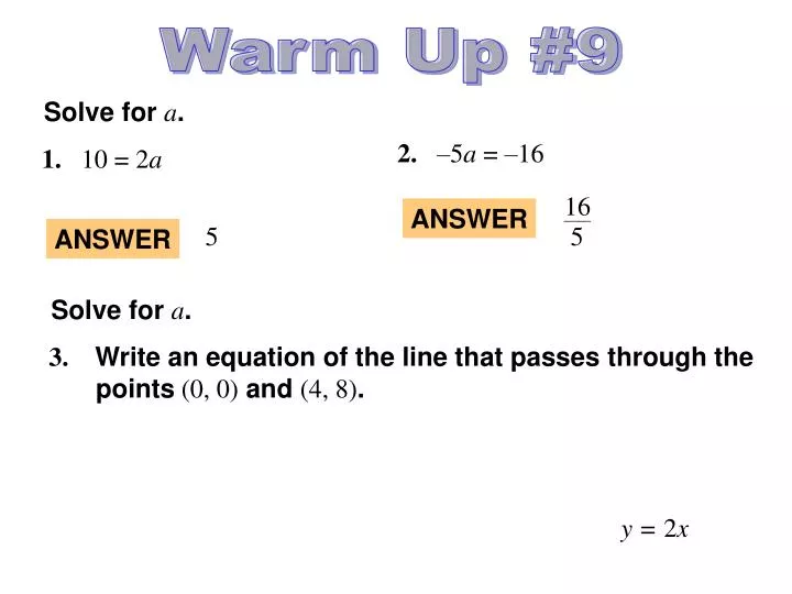
16. 5. Warm Up #9. Solve for a. 2. –5 a = –16. 1. 10 = 2 a. ANSWER. 5. ANSWER. Solve for a. 3. Write an equation of the line that passes through the points (0, 0) and (4, 8). y = 2 x. Main Concept.

E N D
16 5 Warm Up #9 Solve for a. 2. –5a = –16 1. 10 = 2a ANSWER 5 ANSWER Solve for a. 3. Write an equation of the line that passes through the points (0, 0) and (4, 8). y = 2x
Substituting –2 for ain y = axgives the direct variation equation y = –2x. EXAMPLE 1 Write and graph a direct variation equation Write and graph a direct variation equation that has (–4, 8) as a solution. Use the given values of xand yto find the constant of variation. y= ax Write direct variation equation. 8 = a(–4) Substitute 8 for yand – 4 for x. –2 = a Solve for a.
ANSWER y = – 3x. (3, –9) for Example 1 GUIDED PRACTICE Write and graph a direct variation equation that has the given ordered pair as a solution. y = ax -9 = a(3) -3 = a
(–7, 4) for Example 1 GUIDED PRACTICE Write and graph a direct variation equation that has the given ordered pair as a solution. y = ax 4 = a(-7) -4/7 = a y = -4/7x
EXAMPLE 2 Write and apply a model for direct variation Meteorology Hailstones form when strong updrafts support ice particles high in clouds, where water droplets freeze onto the particles. The diagram shows a hailstone at two different times during its formation.
After t = 20 minutes, the predicted diameter of the hailstone is d = 0.0625(20) = 1.25 inches. EXAMPLE 2 Write and apply a model for direct variation a. Write an equation that gives the hailstone’s diameter d(in inches) after tminutes if you assume the diameter varies directly with the time the hailstone takes to form. d=at b. Using your equation from part (a), predict the diameter of the hailstone after 20 minutes. d=at 0.75=a(12) 0.0625 = a An equation that relates tand dis d = 0.0625t.
Correlation: +1 Correlation: -1 Correlation: 0 Correlation: +1/2 Correlation: -1/2
EXAMPLE 1 Describe correlation Describe the correlation shown by each scatter plot. Positive or Negative Positive Correlation Negative Correlation The first scatter plot shows a positive correlation, because as the number of cellular phone subscribers increased, the number of cellular service regions tended to increase. The second scatter plot shows a negative correlation, because as the number of cellular phone subscribers increased, corded phone sales tended to decrease.
a. a. The scatter plot shows a clear but fairly weak negative correlation. So, r is between 0 and –1, but not too close to either one. The best estimate given is r=–0.5. (The actual value is r–0.46.) EXAMPLE 2 Estimate correlation coefficients Tell whether the correlation coefficient for the data is closest to –1, –0.5, 0, 0.5, or 1. SOLUTION
b. b. The scatter plot shows approximately no correlation. So, the best estimate given is r=0. (The actual value is r –0.02.) EXAMPLE 2 Estimate correlation coefficients SOLUTION
c. c. The scatter plot shows a strong positive correlation. So, the best estimate given is r = 1. (The actual value is r0.98.) EXAMPLE 2 Estimate correlation coefficients SOLUTION
1. for Examples 1 and 2 GUIDED PRACTICE For each scatter plot, (a) tell whether the data have a positive correlation, a negative correlation, or approximately no correlation, and (b) tell whether the correlation coefficient is closest to –1, – 0.5, 0, 0.5, or 1. ANSWER (a)positive correlation (b)r = 0.5
2. for Examples 1 and 2 GUIDED PRACTICE For each scatter plot, (a) tell whether the data have a positive correlation, a negative correlation, or approximately no correlation, and (b) tell whether the correlation coefficient is closest to –1, – 0.5, 0, 0.5, or 1. ANSWER (a)negative correlation (b)r = –1
3. for Examples 1 and 2 GUIDED PRACTICE For each scatter plot, (a) tell whether the data have a positive correlation, a negative correlation, or approximately no correlation, and (b) tell whether the correlation coefficient is closest to –1, –0.5, 0, 0.5, or 1. ANSWER (a)no correlation (b)r = 0
EXAMPLE 3 Approximate a best-fitting line Alternative-fueled Vehicles The table shows the number y (in thousands) of alternative-fueled vehicles in use in the United States xyears after 1997. Approximate the best-fitting line for the data. This will be very important for our project next week!
EXAMPLE 3 Approximate a best-fitting line SOLUTION STEP 1 Draw a scatter plot of the data. STEP 2 Sketch the line that appears to best fit the data. One possibility is shown.
248 548 – 300 m = = 41.3 6 7 – 1 EXAMPLE 3 Approximate a best-fitting line STEP 3 Choose two points that appear to lie on the line. For the line shown, you might choose (1,300), which is not an original data point, and (7,548), which is an original data point. STEP 4 Write an equation of the line. First find the slope using the points (1,300) and (7,548).
y 41.3x + 259 ANSWER An approximation of the best-fitting line is y=41.3x+259. EXAMPLE 3 Approximate a best-fitting line Use point-slope form to write the equation. Choose (x1, y1) = (1,300). y – y1 = m(x – x1) Point-slope form y – 300 = 41.3(x – 1) Substitute for m,x1, and y1. Simplify.
y = 41.3x + 259 = 41.3(13) + 259 796 EXAMPLE 4 Use a line of fit to make a prediction Use the equation of the line of fit from Example 3 to predict the number of alternative-fueled vehicles in use in the United States in 2010. SOLUTION Because 2010 is 13 years after 1997, substitute 13 for x in the equation from Example 3.
ANSWER You can predict that there will be about 796,000 alternative-fueled vehicles in use in the United States in 2010. EXAMPLE 4 Use a line of fit to make a prediction
Classwork:Worksheet 2-5 (1-21 odd) Worksheet 2-6 (1-10 all)