Download
1 / 4
40 likes | 137 Views
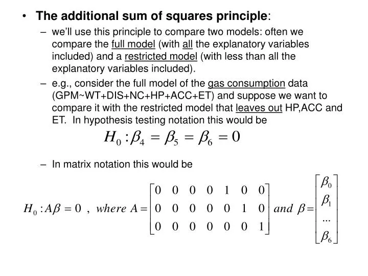
The additional sum of squares principle : we’ll use this principle to compare two models: often we compare the full model (with all the explanatory variables included) and a restricted model (with less than all the explanatory variables included).

E N D
Theadditional sum of squares principle: • we’ll use this principle to compare two models: often we compare the full model (with all the explanatory variables included) and a restricted model (with less than all the explanatory variables included). • e.g., consider the full model of the gas consumption data (GPM~WT+DIS+NC+HP+ACC+ET) and suppose we want to compare it with the restricted model that leaves out HP,ACC and ET. In hypothesis testing notation this would be • In matrix notation this would be
be able to explain what the “reject the null” and “fail to reject the null” mean in this case... • the test of this hypothesis is done by using the additional sum of squares F-statistic ; it uses this fact: Suppose W is regression model that predicts y using a set of explanatory variables and suppose w is another model predicting the same response, but with a subset of explanatory variables contained in W. Then W has a smaller error sum of squares than w . (look at the simple linear regression case...). So the additional error sum of squares, gained by including only the explanatory variables in w is SSEw – SSEW . Intuitively, if this is small, (not significant) then we could use the smaller model since the additional explanatory variables don’t seem to be contributing much reduction in the error sum of squares. We test significance with the following F-statistic:
Here, p=# expl. vars in W and q=#expl. vars in w . The resulting quotient has an F-distribution, assuming the null hypothesis is true. The null hypothesis being tested is where the number of parameters being tested here is q (out of the total of p+1)... So let’s try this on the problem we mentioned on page 1 testing in the gas consumption data. Recall, n=38, p=number of expl. vars in full model = 6, q=number of expl. vars in the reduced model = 3. Using R again, compute the SSE for each model and get: SSEW = 3.037351 on 31 d.f. (38-6-1) and SSEw = 4.805601 on 34 d.f. (38-3-1). Thus the F-statistic to test the above null hypothesis is given by (4.805601-3.037351)/(34-31) / (3.037351/31) = 6.015741 . The tabulated value (0.01) is ~4.51. Clearly we reject the null hypothesis and at least one of beta3,4, or 5 is not zero.
see R#7 for some other examples of this important test statistic and some short-cut ways to compute them. Two other examples is a test of all parameters (except the intercept) = 0 and the individual parameters =0 • try this out on some of your other example datasets... • finish reading through section 4.4 – we’ll pick up after this next time. Note that the reading here is tough – make sure you know and understand the summaries I’m providing in these notes and in the R-notes...