Download
1 / 67
680 likes | 814 Views
Lecture 9: Multiscale Bio-Modeling and Visualization Tissue Models II: Contouring 3D Images. Chandrajit Bajaj http://www.cs.utexas.edu/~bajaj. Imaging Modalities. Contouring for Models and Visualization. The Isocontour Computation Problem. Input: Scalar Field F defined on a mesh

E N D
Lecture 9: Multiscale Bio-Modeling and VisualizationTissue Models II: Contouring 3D Images Chandrajit Bajaj http://www.cs.utexas.edu/~bajaj Center for Computational Visualization Institute of Computational and Engineering Sciences Department of Computer Sciences University of Texas at Austin
Imaging Modalities Center for Computational Visualization Institute of Computational and Engineering Sciences Department of Computer Sciences University of Texas at Austin
Contouring for Models and Visualization Center for Computational Visualization Institute of Computational and Engineering Sciences Department of Computer Sciences University of Texas at Austin
The Isocontour Computation Problem • Input: • Scalar Field F defined on a mesh • MultipleIsovalues win unpredictable order • Output (for each isovalue w):Contour C(w) = {x | F(x) = w} Center for Computational Visualization Institute of Computational and Engineering Sciences Department of Computer Sciences University of Texas at Austin
The Isocontour Computation Problem an an Isosurface of isovalue ah Lower Bound } an an Input size n m+log(n) Output size m Mesh The search for ah takes at least log(n) a3 a2 a1 a3 a2 a3 a1, a2, a3, a4, … , an a2 a1 a1 Center for Computational Visualization Institute of Computational and Engineering Sciences Department of Computer Sciences University of Texas at Austin
Related Work Search Space Geometric Value Giles/Haimes (min-sorted ranges) Lorenson/Cline (Marching Cubes) Shen/Livnat/Johnson/Hansen (LxL lattice) Wilhelms/Van Gelder (octree) Gallagher(span decomposed into backets) Cell by Cell Shen/Johnson (hierachical min-max ranges) Cignoni/Montani/Puppo/Scopigno Livnat/Shen/Johnson (kd-tree) Contouring Strategy Howie/Blake(propagation) van Kreveld Itoh/Koyamada (extrema graph) Bajaj/Pascucci/Schikore Itoh/Yamaguchi/Koyamada (volume thinnig) Mesh Propagation van Kreveld /van Oostrum/Bajaj/Pascucci/Schikore Center for Computational Visualization Institute of Computational and Engineering Sciences Department of Computer Sciences University of Texas at Austin
Temporal CoherenceShen View DependentLivnat/Hansen AdaptiveZhou/Chen/Kaufman Parallel (SIMD)Hansen/Hinker Parallel(cluster)Ellsiepen Out-of-coreChiang/Silva/Schroeder Parallel ray tracingParker/Shirley/Livnat/Hansen/Sloan Parallel & Out-of-core-Bajaj/Pascucci/Thompson/Zhang -Zhang/Bajaj -Zhang/Bajaj/Ramachandran Temporal-coherenceSutton/Hansen Addtl Related Work (Parallel) Center for Computational Visualization Institute of Computational and Engineering Sciences Department of Computer Sciences University of Texas at Austin
Optimal Single-Resolution Isocontouring The basic scheme (fmin,fmax) Preprocessing: For each cell c in M Enter its range of function values into an interval-tree Center for Computational Visualization Institute of Computational and Engineering Sciences Department of Computer Sciences University of Texas at Austin
Optimal Single-Resolution Isocontouring The basic scheme Isocontour query W For each interval containing W Compute the portion of isocontour in the corresponding cell (fmin,fmax) Center for Computational Visualization Institute of Computational and Engineering Sciences Department of Computer Sciences University of Texas at Austin
Optimal Single-Resolution Isocontouring The basic scheme Isocontour query W Complexity: m + log(n) Optimal but impracticalbecause of the size of theinterval-tree (fmin,fmax) Center for Computational Visualization Institute of Computational and Engineering Sciences Department of Computer Sciences University of Texas at Austin
Optimal Single-Resolution Isocontouring Seed Set Optimization For each connected componentwe need only one cell (and then propagate by adjacency in the mesh) Seed Set: a set of cells intersectingevery connected component of every isocontour (fmin,fmax) Center for Computational Visualization Institute of Computational and Engineering Sciences Department of Computer Sciences University of Texas at Austin
Optimal Single-Resolution Isocontouring The basic scheme (fmin,fmax) Preprocessing (revised): For each cell c in a Seed Set Enter its range of function values into an interval-tree Center for Computational Visualization Institute of Computational and Engineering Sciences Department of Computer Sciences University of Texas at Austin
Optimal Single-Resolution Isocontouring Seed SetGeneration (k seeds from n cells) • 238 seed cells • 0.01 seconds Range Sweep Domain Sweep Responsibility Propagation Time O(n) O(n) O(n log n) O(k) O(n) O(k) Space ? 2 kmin ? k = 59 seed cells 1.02 seconds 177 seed cells 0.05 seconds Test Center for Computational Visualization Institute of Computational and Engineering Sciences Department of Computer Sciences University of Texas at Austin
Optimal Single-Resolution Isocontouring Seed Set Generation 720000 # C e l l s 29356 144.51 T i m e (s) Eagle Pass Terrain 1.4 M total cells 7151 17.24 16.24 1872 4.40 C l i m b P r o p S w e e p C h e c k e r Center for Computational Visualization Institute of Computational and Engineering Sciences Department of Computer Sciences University of Texas at Austin
Optimal Single-Resolution Isocontouring 20 25 Contour tree 0 25 20 0 Center for Computational Visualization Institute of Computational and Engineering Sciences Department of Computer Sciences University of Texas at Austin
Optimal Single-Resolution Isocontouring Minimal Seed Set Contour Tree f Center for Computational Visualization Institute of Computational and Engineering Sciences Department of Computer Sciences University of Texas at Austin
Optimal Single-Resolution Isocontouring Contour Tree (local minima) Minimal Seed Set f Center for Computational Visualization Institute of Computational and Engineering Sciences Department of Computer Sciences University of Texas at Austin
Optimal Single-Resolution Isocontouring Contour Tree (local maxima) Minimal Seed Set f Center for Computational Visualization Institute of Computational and Engineering Sciences Department of Computer Sciences University of Texas at Austin
Optimal Single-Resolution Isocontouring Contour Tree Minimal Seed Set Each seed cell corresponds to a monotonic path on the contour tree f Center for Computational Visualization Institute of Computational and Engineering Sciences Department of Computer Sciences University of Texas at Austin
Optimal Single-Resolution Isocontouring Contour Tree Minimal Seed Set For a minimal seed set each seed cell corresponds to a path that is not covered by any over seed cell f Center for Computational Visualization Institute of Computational and Engineering Sciences Department of Computer Sciences University of Texas at Austin
Optimal Single-Resolution Isocontouring Contour Tree Minimal Seed Set Current isovalue Each connected component of any isocontour corresponds exactly to one point of the contour tree f Center for Computational Visualization Institute of Computational and Engineering Sciences Department of Computer Sciences University of Texas at Austin
Optimal Single-Resolution Isocontouring Range sweep Center for Computational Visualization Institute of Computational and Engineering Sciences Department of Computer Sciences University of Texas at Austin
Optimal Single-Resolution Isocontouring • The number of seeds selected is the minimum plus the number of local minima. Center for Computational Visualization Institute of Computational and Engineering Sciences Department of Computer Sciences University of Texas at Austin
Optimal Single-Resolution Isocontouring Seed set of a 3D scalar field Center for Computational Visualization Institute of Computational and Engineering Sciences Department of Computer Sciences University of Texas at Austin
Quantitative Analysis I • Consider a terrain of which you want to compute the length of each isocontour and the area contained inside each isocontour. Center for Computational Visualization Institute of Computational and Engineering Sciences Department of Computer Sciences University of Texas at Austin
Quantitative Analysis II(signature computation) The length of each contour is a c0spline function. • The area inside/outside each isocontour is a C1spline function. Center for Computational Visualization Institute of Computational and Engineering Sciences Department of Computer Sciences University of Texas at Austin
Quantitative Analysis III(signature computation) • In general the size of each isocontour of a scalar field of dimension d is a spline function of d-2 continuity. • The size of the region inside/outside is given by a spline function of d-1 continuity Center for Computational Visualization Institute of Computational and Engineering Sciences Department of Computer Sciences University of Texas at Austin
The Contour Spectrum Graphical User Interface for Static Data • The horizontal axis spans the scalar values • Plot of a set of signatures (length, area, gradient ...) as functions of the scalar value . • Vertical axis spans normalized ranges of each signature. • White vertical bars mark current selected isovalues. Center for Computational Visualization Institute of Computational and Engineering Sciences Department of Computer Sciences University of Texas at Austin
The Contour SpectrumGraphical User Interface for time varying data high (,t ) --> c The color c is mapped to the magnitude of a signature function of time tand isovalue The horizontal axis spans the scalar value dimension The vertical axis spans the time dimension t c magnitude t low Center for Computational Visualization Institute of Computational and Engineering Sciences Department of Computer Sciences University of Texas at Austin
Spectrum-based Contouring (CT scan of an engine model) • The contour spectrum allows the development of an adaptive ability to separate interesting isovalues from the others. Center for Computational Visualization Institute of Computational and Engineering Sciences Department of Computer Sciences University of Texas at Austin
Spectrum-based Contouring (foot of the Visible Human) Center for Computational Visualization Institute of Computational and Engineering Sciences Department of Computer Sciences University of Texas at Austin
Visualization of Electrostatic Potential(a view inside the data) Center for Computational Visualization Institute of Computational and Engineering Sciences Department of Computer Sciences University of Texas at Austin
Progressive Isocontouring of Images Center for Computational Visualization Institute of Computational and Engineering Sciences Department of Computer Sciences University of Texas at Austin
Progressive Isocontouring cascaded multi-resolutionon-line algorithms Isocontouring Mesh Refinement Display Center for Computational Visualization Institute of Computational and Engineering Sciences Department of Computer Sciences University of Texas at Austin
Progressive Isocontouring • Input: • hierarchical mesh (e.g. generated by edge bisection) • an isovalue • Output: • a hierarchical representation of the required isosurface • the input mesh must be traversed from the coarse level to the fine level • as the input mesh is partially traversed the output contour hierarchy must be generated Center for Computational Visualization Institute of Computational and Engineering Sciences Department of Computer Sciences University of Texas at Austin
Progressive Isocontouring Edge Bisection Center for Computational Visualization Institute of Computational and Engineering Sciences Department of Computer Sciences University of Texas at Austin
Progressive Isocontouring • Local refinement:only the cells incident to the split edge are refined. • Adaptivity without “temporary” subdivision. Center for Computational Visualization Institute of Computational and Engineering Sciences Department of Computer Sciences University of Texas at Austin
Progressive Isocontouring The 1D case isovalue isovalue Center for Computational Visualization Institute of Computational and Engineering Sciences Department of Computer Sciences University of Texas at Austin
Progressive Isocontouring 2D case 16 cases can be reduced immediately to 8 by +/- symmetry - + + + (1) (2) (3) (4) (5) (1’) (4’) (2’) Center for Computational Visualization Institute of Computational and Engineering Sciences Department of Computer Sciences University of Texas at Austin
Vertex Move Progressive Isocontouring Vertex Move Vertex Split Vertex Split Vertex Move Vertex Split Vertex Split Vertex Split (2) (3) (1) (1) Center for Computational Visualization Institute of Computational and Engineering Sciences Department of Computer Sciences University of Texas at Austin
Vertex Split Progressive Isocontouring Vertex Split Vertex Split Vertex Split New Loop Edge Flip Vertex Split Vertex Split (4) (4) (5) (3) Center for Computational Visualization Institute of Computational and Engineering Sciences Department of Computer Sciences University of Texas at Austin
Progressive Isocontouring Vertex Move Vertex Split Vertex Split Vertex Move Center for Computational Visualization Institute of Computational and Engineering Sciences Department of Computer Sciences University of Texas at Austin
Progressive Isocontouring Vertex Move Vertex Split Vertex Split Vertex Split Center for Computational Visualization Institute of Computational and Engineering Sciences Department of Computer Sciences University of Texas at Austin
Progressive Isocontouring Vertex Split New Loop Vertex Split Center for Computational Visualization Institute of Computational and Engineering Sciences Department of Computer Sciences University of Texas at Austin
Progressive Isocontouring Vertex Flip Vertex Flip Vertex Split Vertex Split Vertex Split Center for Computational Visualization Institute of Computational and Engineering Sciences Department of Computer Sciences University of Texas at Austin
Progressive Isocontouring Center for Computational Visualization Institute of Computational and Engineering Sciences Department of Computer Sciences University of Texas at Austin
Progressive Isocontouring Center for Computational Visualization Institute of Computational and Engineering Sciences Department of Computer Sciences University of Texas at Austin
Progressive Isocontouring Center for Computational Visualization Institute of Computational and Engineering Sciences Department of Computer Sciences University of Texas at Austin
Higher Order Contouring with A-patches Center for Computational Visualization Institute of Computational and Engineering Sciences Department of Computer Sciences University of Texas at Austin
A-patches in BB-form • Given tetrahedron vertices pi=(xi,yi,zi), i=1,2,3,4, • a is barycentric coordinates of p=(x,y,z) : • function f(p) of degree n can be expressed in Bernstein-Bezier form : • Algebraic surface patch(A-patch) within the tet is defined as f(p)=0. Center for Computational Visualization Institute of Computational and Engineering Sciences Department of Computer Sciences University of Texas at Austin