Download
1 / 44
440 likes | 636 Views
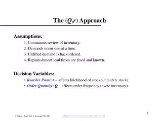
The ( Q , r ) Approach. Assumptions: 1. Continuous review of inventory. 2. Demands occur one at a time. 3. Unfilled demand is backordered. 4. Replenishment lead times are fixed and known. Decision Variables: Reorder Point : r – affects likelihood of stockout ( safety stock ).

E N D
The (Q,r) Approach • Assumptions: 1. Continuous review of inventory. 2. Demands occur one at a time. 3. Unfilled demand is backordered. 4. Replenishment lead times are fixed and known. • Decision Variables: • Reorder Point:r – affects likelihood of stockout (safety stock). • Order Quantity:Q – affects order frequency (cycle inventory).
Inventory vs Time in (Q,r) Model Inventory Q r l Time
Base Stock Model Assumptions • 1. There is no fixed cost associated with placing an order. • 2. There is no constraint on the number of orders that can be placed per year.
Base Stock Notation • Q = 1, order quantity (fixed at one) • r = reorder point • R = r +1, base stock level • l = delivery lead time • q = mean demand during l • = std dev of demand during l • p(x) = Prob{demand during lead time lequals x} • G(x) = Prob{demand during lead time l is less than or equal to x} • h = unit holding cost • b = unit backorder cost • S(R) = average fill rate (service level) • B(R) = average backorder level • I(R) = average on-hand inventory level
Inventory Balance Equations • Balance Equation: • inventory position = on-hand inventory - backorders + orders • Under Base Stock Policy • inventory position = R
Service Level (Fill Rate) • Let: X = (random) demand during lead time l • so E[X] = . Consider a specific replenishment order. Since inventory position is always R, the only way this item can stock out is if X R. • Expected Service Level:
Backorder Level • Note:At any point in time, number of orders equals number demands during last l time units (X) so from our previous balance equation: • R = on-hand inventory - backorders + orders • on-hand inventory - backorders = R - X • Note: on-hand inventory and backorders are never positive at the same time, so if X=x, then • Expected Backorder Level: simpler version for spreadsheet computing
Inventory Level • Observe: • on-hand inventory - backorders = R-X • E[X] = from data • E[backorders] = B(R) from previous slide • Result: • I(R) = R - + B(R)
Base Stock Example l = one month q = 10 units (per month) Assume Poisson demand, so Note: Poisson demand is a good choice when no variability data is available.
Base Stock Example Results • Service Level: For fill rate of 90%, we must set R-1= r =14, so R=15 and safety stock s = r- = 4. Resulting service is 91.7%. • Backorder Level: • B(r) = 0.187 • Inventory Level: • I(R) = R - + B(R) = 15 - 10 + 0.187 = 5.187
“Optimal” Base Stock Levels • Objective Function: Y(R) = hI(R) + bB(R) = h(R-+B(R)) + bB(R) = h(R- ) + (h+b)B(R) • Solution: if we assume G is continuous, we can use calculus to get holding plus backorder cost Implication: set base stock level so fill rate is b/(h+b). Note: R* increases in b and decreases in h.
Base Stock Normal Approximation • If G is normal(,), then • where (z)=b/(h+b). So • R* = + z Note: R* increases in and also increases in provided z>0.
“Optimal” Base Stock Example • Data:Approximate Poisson with mean 10 by normal with mean 10 units/month and standard deviation 10 = 3.16 units/month. Set h=$15, b=$25. • Calculations: • since (0.32) = 0.625, z=0.32 and hence • R* = + z = 10 + 0.32(3.16) = 11.01 11 • Observation:from previous table fill rate is G(10) = 0.583, so maybe backorder cost is too low.
Inventory Pooling • Situation: • n different parts with lead time demand normal(,) • z=2 for all parts (i.e., fill rate is around 97.5%) • Specialized Inventory: • base stock level for each item = + 2 • total safety stock = 2n • Pooled Inventory: suppose parts are substitutes for one another • lead time demand is normal (n,n ) • base stock level (for same service) = n +2 n • ratio of safety stock to specialized safety stock = 1/ n cycle stock safety stock
Effect of Pooling on Safety Stock Conclusion: cycle stock is not affected by pooling, but safety stock falls dramatically. So, for systems with high safety stock, pooling (through product design, late customization, etc.) can be an attractive strategy.
Pooling Example • PC’s consist of 6 components (CPU, HD, CD ROM, RAM, removable storage device, keyboard) • 3 choices of each component: 36 = 729 different PC’s • Each component costs $150 ($900 material cost per PC) • Demand for all models is Poisson distributed with mean 100 per year • Replenishment lead time is 3 months (0.25 years) • Use base stock policy with fill rate of 99%
Pooling Example - Stock PC’s • Base Stock Level for Each PC: = 100 0.25 = 25, so using Poisson formulas, • G(R-1) 0.99 R = 38 units • On-Hand Inventory for Each PC: • I(R) = R - + B(R) = 38 - 25 + 0.023 = 13.023 units • Total (Approximate) On-Hand Inventory : • 13.023 729 $900 = $8,544,390
Pooling Example - Stock Components 729 models of PC 3 types of each comp. • Necessary Service for Each Component: • S = (0.99)1/6 = 0.9983 • Base Stock Level for Components: = (100 729/3)0.25 = 6075, so • G(R-1) 0.9983 R = 6306 • On-Hand Inventory Level for Each Component: • I(R) = R - + B(R) = 6306-6075+0.0363 = 231.0363 units • Total Safety Stock: • 231.0363 18 $150 = $623,798 93% reduction!
Base Stock Insights 1. Reorder points control the probability of stockouts by establishing safety stock. 2. The “optimal” fill rate is an increasing function of the backorder cost and a decreasing function of the holding cost. We can use either a service constraint or a backorder cost to determine the appropriate base stock level. 3. Base stock levels in multi-stage production systems are very similar to kanban systems and therefore the above insights apply to those systems as well. 4. Base stock model allows us to quantify benefits of inventory pooling.
The Single Product (Q,r) Model • Motivation: Either 1. Fixed cost associated with replenishment orders and cost per backorder. 2. Constraint on number of replenishment orders per year and service constraint. • Objective: Under (1) As in EOQ, this makes batch production attractive.
(Q,r) Notation (cont.) • Decision Variables: • Performance Measures:
Inventory and Inventory Position for Q=4, r=4 Inventory Position uniformly distributed between r+1=5 and r+Q=8
Costs in (Q,r) Model • Fixed Setup Cost: AF(Q) • Stockout Cost: kD(1-S(Q,r)), where k is cost per stockout • Backorder Cost: bB(Q,r) • Inventory Carrying Costs: cI(Q,r)
Fixed Setup Cost in (Q,r) Model • Observation: since the number of orders per year is D/Q,
Stockout Cost in (Q,r) Model • Key Observation: inventory position is uniformly distributed between r+1 and r+Q. So, service in (Q,r) model is weighted sum of service in base stock model. • Result: Note: this form is easier to use in spreadsheets because it does not involve a sum.
Service Level Approximations • Type I (base stock): • Type II: Note: computes number of stockouts per cycle, underestimates S(Q,r) Note: neglects B(r,Q) term, underestimates S(Q,r)
Backorder Costs in (Q,r) Model • Key Observation: B(Q,r) can also be computed by averaging base stock backorder level function over the range [r+1,r+Q]. • Result: Notes: 1. B(Q,r) B(r) is a base stock approximation for backorder level. 2. If we can compute B(x) (base stock backorder level function), then we can compute stockout and backorder costs in (Q,r) model.
Inventory Costs in (Q,r) Model • Approximate Analysis: on average inventory declines from Q+s to s+1 so • Exact Analysis: this neglects backorders, which add to average inventory since on-hand inventory can never go below zero. The corrected version turns out to be
(Q,r) Model with Backorder Cost • Objective Function: • Approximation: B(Q,r) makes optimization complicated because it depends on both Q and r. To simplify, approximate with base stock backorder formula, B(r):
Results of Approximate Optimization • Assumptions: • Q,r can be treated as continuous variables • G(x) is a continuous cdf • Results: Note: this is just the EOQ formula Note: this is just the base stock formula if G is normal(,), where (z)=b/(h+b)
(Q,r) Example D = 14 units per year c = $150 per unit h = 0.1 × 150 = $15 per unit l= 45 days q = (14 × 45)/365 = 1.726 units during replenishment lead time A = $10 b = $40 Demand during lead time is Poisson
Observations on Example • Orders placed at rate of 3.5 per year • Fill rate fairly high (90.4%) • Very few outstanding backorders (0.049 on average) • Average on-hand inventory just below 3 (2.823)
Varying the Example • Change: suppose we order twice as often so F=7 per year, then Q=2 and: • which may be too low, so increase r from 2 to 3: • This is better. For this policy (Q=2, r=4) we can compute B(2,3)=0.026, I(Q,r)=2.80. • Conclusion: this has higher service and lower inventory than the original policy (Q=4, r=2). But the cost of achieving this is an extra 3.5 replenishment orders per year.
(Q,r) Model with Stockout Cost • Objective Function: • Approximation: Assume we can still use EOQ to compute Q* but replace S(Q,r) by Type II approximation and B(Q,r) by base stock approximation:
Results of Approximate Optimization • Assumptions: • Q,r can be treated as continuous variables • G(x) is a continuous cdf • Results: Note: this is just the EOQ formula Note: another version of base stock formula (only z is different) if G is normal(,), where (z)=kD/(kD+hQ)
Backorder vs. Stockout Model • Backorder Model • when real concern is about stockout time • because B(Q,r) is proportional to time orders wait for backorders • useful in multi-level systems • Stockout Model • when concern is about fill rate • better approximation of lost sales situations (e.g., retail) • Note: • We can use either model to generate frontier of solutions • Keep track of all performance measures regardless of model • B-model will work best for backorders, S-model for stockouts
Lead Time Variability • Problem: replenishment lead times may be variable, which increases variability of lead time demand. • Notation: L = replenishment lead time (days), a random variable l= E[L] = expected replenishment lead time (days) L= std dev of replenishment lead time (days) Dt = demand on day t, a random variable, assumed independent and identically distributed d = E[Dt] = expected daily demand D= std dev of daily demand (units)
Including Lead Time Variability in Formulas • Standard Deviation of Lead Time Demand: • Modified Base Stock Formula (Poisson demand case): if demand is Poisson Inflation term due to lead time variability Note: can be used in any base stock or (Q,r) formula as before. In general, it will inflate safety stock.
Single Product (Q,r) Insights • Basic Insights: • Safety stock provides a buffer against stockouts. • Cycle stock is an alternative to setups/orders. • Other Insights: 1. Increasing D tends to increase optimal order quantity Q. 2. Increasing q tends to increase the optimal reorder point. (Note: either increasing D or l increases q.) 3. Increasing the variability of the demand process tends to increase the optimal reorder point (provided z > 0). 4. Increasing the holding cost tends to decrease the optimal order quantity and reorder point.