Download
1 / 19
190 likes | 424 Views
Giorgi Japaridze Logic. First Order Logic. Episode 5. Propositional logic versus first-order (predicate) logic The universe of discourse Constants, variables, terms and valuations Predicates as generalized propositions

E N D
Giorgi Japaridze Logic First Order Logic Episode 5 • Propositional logic versus first-order (predicate) logic • The universe of discourse • Constants, variables, terms and valuations • Predicates as generalized propositions • Boolean operations as operations on predicates • Substitution of variables • Quantifiers • The language of first-order logic • Interpretation, truth and validity • The undecidability of the validity problem • A Gentzen-style deductive system • Soundness and Gödel’s completeness • Peano arithmetic and Gödel’s incompleteness 0
5.1 The language of propositional logic is very poor and does not allow us to talk about many things that we would like to be able to talk about. That is because propositional logic fails to “look inside propositions” and see any further structure in them. For example, propositional logic would not see any connection between “Bob likes Jane” and “There is someone who likes Jane”, even though one statement logically implies the other. Propositional logic versus predicate logic This limitation of expressive power is overcome in predicate logic, which is also called first-order logic. It is based not just on propositions, but on predicates (=relations). Propositions are simple special cases of predicates. Hence, propositional logic is just a simple fragment of the more expressive predicate logic. In a sense, the expressive power of first-order logic is universal: it allows us to talk about virtually anything. Note: In this episode, first-order logic will be presented in a way which may seem quite different from the treatments that you have probably seen elsewhere. Yet, our approach is equivalent to the more traditional ones.
5.2 Relations are always considered in the context of some set. For example, when we mention <, we may say that we mean it as a binary relation on the set N of natural numbers. This formally means that < is a subset of NN. Such a context-setting set (in this example N) is said to be the universe of discourse. The universe of discourse When applying first-order logic, we always have some universe of discourse in mind. For example, if first-order logic is used for building a formal arithmetic, the universe of discourse would be N. And if logic is used for a biological classification system, the universe of discourse would contain (the names of) all plants and animals. In our treatment, we assume that the universe of discourse is always N. There is no (much) loss of generality in doing so. After all, plants, people, chemical elements, rational numbers --- all objects that have or can have names --- can be encoded as natural numbers.
5.3 Constants, variables, terms and valuations We identify the elements of our universe of discourse with their decimal representations, and call the elements of {0,1,2,...,17,... } constants. The letters a, b, c, d will be typically used as metavariables for constants. Next, we fix another countably infinite set of expressions and call its elements variables. The letters x,y,z will be typically used as metavariables for variables. A term means either a variable or a constant. The letter t will be typically used as a metavariable for terms. A valuation is any function that assigns a constant to each variable. The letter e will be typically used as a metavariable for valuations. We extend the domain of each valuation e to all terms by stipulating that, for any constant c, e(c)=c.
5.4 Predicates revisited From now on, by a predicate we will always mean a function p that assigns a value e[p]{⊤,⊥} (“true” or “false”) to each valuation e. Note that we write e[p] instead of p(e). When e[p]=⊤ , we say that predicate p is true ate. And when e[p]=⊥, we say that p is false ate. For example, the predicate “x is even”, or Even(x), is defined by e[Even(x)] = ⊤ife(x)is even; ⊥ otherwise. And the predicate “x is greater than y”, or x>y, is defined by e[x>y] = ⊤ife(x)>e(y); ⊥ otherwise.
5.5 Constant predicates; propositions as special cases of predicates We say that a predicate p is constant if its value does not depend on valuation. That is, p is constant iff, for any two valuations e and e’, we have e[p]=e’[p]. x>y x>x x>0 x0 2+2=5 no yes Examples. Are the following predicates constant? no yes yes The last example above illustrates that propositions are nothing but constant predicates. In general, propositional logic is nothing but first-order logic restricted to constant predicates. We say that a predicate pdepends on a variable x iff there are two valuations e and e’ such that: (a) e and e’ agree on all variables except x, and (b) e[p]e’[p]. Constant predicates (propositions) thus do not depend on any variables.
5.6 Boolean operations as operations on predicates In Episode 4, Boolean operations were defined as operations on propositions, i.e. functions of the type {propositions}n{propositions} (n=0, n=1 or n=2). They easily extend to operations on predicates, i.e. functions of the type {predicates}n{predicates}, by the following definition: For every valuation e and all predicates p and q: e[p] = (e[p]), i.e., p is true at e iff p is false at e; e[pq] = (e[p]) (e[q]), i.e., pq is true at e iff so are both p and q; e[pq] = (e[p])(e[q]), i.e., pq is true at e iff so is either p or q or both; e[pq] = (e[p])(e[q]), i.e., pq is true at e iff either p is false at e, or q is true at e, or both.
5.7 We often fix a tuple x1,...,xn of pairwise distinct variables for a given predicate p, and write p (when first mentioning it) as p(x1,...,xn). Note: by doing so, we do not necessarily mean that p depends on all of the variables x1,...,xn, or that p does not depend on any other variables. Substitution of variables • When p(x1,...,xn) is as above and t1,...,tn are any terms, p(t1,...,tn) is • written to mean the predicate such that, for any valuation e, we have • e[p(t1,...,tn)]=e’[p(x1,...,xn)], where e’ is the valuation satisfying the • following two conditions: • e’(x1)=e(t1), ..., e’(xn)=e(tn); • e’ agrees with e on all other variables. Example. Let both p(x,y) and q(x) mean “x is a multiple of y”. Then: p(15,3) = p(x,3) = p(y,y) = p(y,z) = q(7) = q(z) = q(y) = “7is a multiple ofy” “15is a multiple of3” =⊤ “x is a multiple of3” “zis a multiple ofy” “yis a multiple ofy” “yis a multiple ofy” =⊤ “yis a multiple ofz”
5.8 Quantifiers • Quantifiers in classical logic are functions of the type • {predicates}{variables} {predicates}. • There are two quantifiers: • universal quantifier, with xpread as “for all x, p”; • existential quantifier, with xp read as “there is x such that p”. They can be defined as “big conjunction” and “big disjunction”: xp(x) = p(0) p(1) p(2) p(3) ... xp(x) = p(0) p(1) p(2) p(3) ... More formally, for any variable x, predicate p(x) and valuation e, we have: e[xp(x)] =⊤iff, for every constant c, e[p(c)]=⊤; e[xp(x)] =⊤iff there is a constant c such thate[p(c)]=⊤.
5.9 Examples Let e be the valuation which assigns 5 to x and assigns 0 to all other variables. Which of the following predicates are true at e and which are false? y<x z<y z(z<x) z(z<y) x(x<x) z(z=y 0<z) true xy(x<y) yx(x<y) yx(xy) xy(xy) 2+3=4 2+3=x true false false true false false true false false true true
5.10 The language of classical first-order logic In addition to the components that the language of propositional logic has, the language of first-order logic contains constants, variables, quantifiers and predicate letters, for which we use p,q,r,s as metavariables. With each predicate letter is associated a natural number called its arity. When the arity of p is n, we say that p is n-ary. An atom of this language is p(t1,...,tn), where p is an n-ary letter and t1,...,tnare any terms. When the arity of p is 0, we write p instead of p(). The atoms of propositional logic remain atoms of first-order logic, as we understand them as 0-ary letters. This includes ⊤and⊥, which are now treated as 0-ary logical predicate letters and hence logical atoms. • Formulas are defined inductively by: • Atoms are formulas; • If F is a formula, so is (F); • If E and F are formulas, so are (E)(F), (E)(F), (E)(F); • If F is a formula and x is a variable, x(F) and x(F) are formulas.
5.11 Free and bound terms; normal formulas An occurrence of a term t in a formula F is said to be bound iff it is in the scope of t or t. Otherwise the occurrence is free. For example, in formula y(p(x,y) xp(x,y)), the first occurrence of x is free while the other occurrences of x, as well as all occurrences of y, are bound. A formula is said to be normal iff no variable has both free and bound occurrences in it. From now on, we will implicitly assume that all formulas that we deal with are normal. That is, from now on, we agree that the word “formula” means “normal formula”.
5.12 An interpretation for first-order logic is a function * that assigns some predicate p*(x1,...,xn) (with the fixed attached tuple x1,...,xn of pairwise distinct variables) to each n-ary nonlogical predicate letter p. Such an interpretation * is said to be admissible for a formula F (or F-admissible) if, for any n-ary predicate letter p of F, the predicate p*(x1,...,xn) assigned to p does not depend on any variables that are not among x1,...,xn but occur in F. In the sequel, we always implicitly assume that the interpretations we consider are admissible for the formulas that we are talking about. Note: In the literature, interpretations are more commonly called models or structures. Interpretations An interpretation * extends to a function *:{formulas}{predicates} by stipulating that: (p(t1,...,tn))*=p*(t1,...,tn); ⊤*=⊤;⊥*=⊥; (F)*=(F*); (EF)*= E*F*; (EF)*= E*F*; (EF)*= E*F*;(xF)*=x(F*); (xF)*=x(F*). Usually we prefer to writeF*(t1,...,tn)instead of(F(t1,...,tn))*.
5.13 Let p be a 3-ary predicate letter, and * be an interpretation that assigns to it the predicate p*(x,y,z) which is true at a given valuation e iff e(x)=e(y)+e(z). What are the meanings of the following formulas (into what predicates do they turn) under this interpretation? Examples p(x,y,z) --- x=y+z p(z,4,y) --- z=4+y p(x,3,5) --- x=3+5 i.e., x=8 p(x,x,x) --- x=x+x i.e., x=0 xy zp(x,y,z) --- zp(z,x,z) --- x=0 xyz(p(x,y,z)p(x,z,y)) --- ⊤ z1z2z3(p(z1,y,y)p(z2,z1,z1)p(z3,z2,z2)p(x,z3,z3)) --- x=16y
5.14 A formula F of first-order logic is said to be valid iff, for every interpretation * and every valuation e, we have e[F*]=⊤. Validity Are the following formulas valid? p(x) No xyq(x,y)yxq(x,y) Yes p(x)p(x) Yes xyq(x,y)yxq(x,y) No x(p(x)p(x)) Yes xy(p(x)p(y)) Yes xy(p(x)p(y)) xp(x)xp(x) No Yes Theorem 5.1. The problem of telling whether a given formula of first-order logic is valid is recursively enumerable but not decidable.
5.15 As in system G2 from Episode 4, we understandsequentsas finite sets of (now first order) formulas. Furthermore, as in Episode 4, we only consider formulas without ⊤, ⊥, and without applied to nonatomic formulas. xF should be understood as xF, and xF as xF. A Gentzen-style deductive system Below are the rules of systemG3. In those rules, G is any set of formulas, E and F are any formulas, x is any variable, H(x) is any formula, t is any term with no bound occurrence in H(x) or G, H(t) is the result of replacing in H(x) all free occurrences of x by t, y is any variable which does not occur in H(x) and G, and H(y) is the result of replacing in H(x) all free occurrences of x by y. Remember also that we require all formulas to be normal (Slide 5.11). For safety, here we also require that sequents, seen as formulas (i.e. disjunctions of their elements) be normal. Axiom -Introduction -Introduction [no premises] G, E G, F G, E, F A G,E,E G, EF G, EF -Introduction -Introduction G, xH(x), H(t) G, H(y) G, xH(x) G, xH(x)
5.16 Examples A yq(z1,y), xq(x,z2), q(z1,z2), q(z1,z2) yq(z1,y), xq(x,z2), q(z1,z2) A G3-proof of xyq(x,y)yxq(x,y). yq(z1,y), xq(x,z2) yq(z1,y), yxq(x,y) xyq(x,y), yxq(x,y) xyq(x,y) yxq(x,y) A xy(p(x)p(y)), p(0), p(z), p(z), p(u) xy(p(x)p(y)), p(0)p(z), p(z)p(u) A G3-proof of xy(p(x)p(y)). xy(p(x)p(y)), p(0)p(z), y(p(z)p(y)) xy(p(x)p(y)), p(0)p(z) xy(p(x)p(y)), y(p(0)p(y)) xy(p(x)p(y))
5.17 The soundness and completeness of G3 Theorem 5.2. For any formula F of first-order logic, we have: Soundness: If F is provable in G3, then F is valid. Completeness: If F is valid, then F is provable in G3. The soundness part of this theorem is relatively easy to prove: just as for G2, it can be done by verifying that all rules preserve validity. The completeness part is harder. It was first proven in 1930 by Kurt Gödel. For that reason, and for the reason of completeness being the more important part, Theorem 5.2 (or the same theorem for any other equivalent deductive system) is called Gödel’s completeness theorem.
5.18 Peano arithmetic Language: =, +, , ’, 0 (a’ means a+1); Underlying logic: an extension of G3 which understands =as the equality predicate. Axioms: 1. xy (x’=y’ x=y) 2. x (x’ 0) 3. x (x+0 = x) 4. xy [x+y’ = (x+y)’] 5. x (x0 = 0) 6. xy [xy’ = (xy)+x] 7. [Q(0) x (Q(x) Q(x’))] xQ(x) Gödel’s Incompleteness Theorem: These axioms are not sufficient to prove every true arithmetical sentence. Neither would be sufficient any bigger set of axioms. Axiom 7 is a scheme,for every formula Q; If Q contains additional variables z1,...,zn, then the whole thing should be prefixed with z1 ... zn This axiom is called the induction scheme